はじめに
『Pythonで学ぶ空間データサイエンス入門』の独学ノートです。本の内容から寄り道してアレコレ考えます。
本を読んだ上で補助的に読んでください。
この記事では、空間隣接行列について、図を使って解説します。
【他の内容】
【今回の内容】
2.1 空間隣接行列の可視化
空間隣接行列(spatial adjacency matrix)を数式とプログラムや図で確認します。
利用するライブラリを読み込みます。
# ライブラリを読込
import geopandas as gpd
from pysal.lib import weights
import numpy as np
import matplotlib.pyplot as plt
import japanize_matplotlib
from matplotlib.animation import FuncAnimation
空間隣接行列の数式表現
まずは、空間隣接行列の定義や計算を数式で確認します。
の(
から
のインデックスで表す)
個の区域に関する空間隣接行列を
とします。
番目と
番目の区域が、隣接していない場合は
、隣接している場合は
で表します。
番目の区域自体(
番目同士の組み合わせの場合)は隣接していない
とします。
隣接関係は区域が入れ替わっても変わらないので、 であり、
は対称行列です。
の
番目の行
の和
や、 番目の列
の和
は、 番目(や
番目)の区域が隣接する区域の数を表します。
ここまでは、空間隣接行列の定義や性質を数式で表現しました。
データの読込
可視化の前に、例として利用する空間データを読み込んで前処理を行います。詳しくは本を参照してください。
「国土数値情報ダウンロードサイト」の行政区域データと地価公示データを読み込みます。
処理コード(クリックで展開)
# ファイルパスを指定
DISTRICT_PATH = 'N03-20230101_27_GML/N03-23_27_230101.shp'
LAND_PATH     = 'L01-23_27_GML/L01-23_27.shp'

# データを読込
gdf_district = gpd.read_file(DISTRICT_PATH, encoding='shift-jis') # 行政区域
gdf_land     = gpd.read_file(LAND_PATH) # 地価公示

# 対象データを取得
gdf_district = gdf_district[['N03_003', 'N03_004', 'N03_007', 'geometry']]
gdf_district.columns = ['city1', 'city2', 'd_code', 'geometry']
gdf_land = gdf_land[['L01_024', 'L01_022', 'L01_006', 'geometry']]
gdf_land.columns = ['address', 'd_code', 'price', 'geometry']

# データを整形
dst_proj = 6668
gdf_district = gdf_district.to_crs(epsg=dst_proj)
gdf_land     = gdf_land.to_crs(epsg=dst_proj) # 空間座標系を再設定
gdf_district['city2_label'] = gdf_district['city2'].str.replace('大阪市|堺市', '', regex=True) # 地名が重なる対策用

# データを加工
gdf_land['log_price'] = np.log(gdf_land['price'])
公示価格の対数をとった列を作成します。その他にも扱いやすいように整形しておきます。
行政区域データと地価公示データをまとめます。
# データを統合
gdf_target = gdf_district.merge(
    gdf_land.groupby('d_code')['log_price'].mean(),
    on='d_code'
)
gdf_target = gdf_target.dissolve(by=['d_code'], as_index=False)
gdf_target['centers'] = gdf_target['geometry'].centroid

# データフレームを整形
gdf_target = gdf_target.reindex(columns=['city1', 'city2', 'd_code', 'geometry', 'centers', 'log_price', 'city2_label'])
gdf_target
| city1 | city2 | d_code | geometry | centers | log_price | city2_label | |
|---|---|---|---|---|---|---|---|
| 0 | 大阪市 | 大阪市都島区 | 27102 | POLYGON ((135.51481 34.72057, 135.51489 34.720... | POINT (135.52721 34.71193) | 12.769969 | 都島区 |
| 1 | 大阪市 | 大阪市福島区 | 27103 | POLYGON ((135.46247 34.6874, 135.46253 34.6879... | POINT (135.47534 34.6939) | 13.214822 | 福島区 |
| 2 | 大阪市 | 大阪市此花区 | 27104 | MULTIPOLYGON (((135.36506 34.6325, 135.35885 3... | POINT (135.42012 34.668) | 12.191524 | 此花区 |
| 3 | 大阪市 | 大阪市西区 | 27106 | POLYGON ((135.46667 34.67284, 135.4642 34.6747... | POINT (135.48375 34.67776) | 13.746399 | 西区 |
| 4 | 大阪市 | 大阪市港区 | 27107 | MULTIPOLYGON (((135.43009 34.64977, 135.4301 3... | POINT (135.45084 34.66032) | 12.410058 | 港区 |
| ... | ... | ... | ... | ... | ... | ... | ... |
| 67 | 泉南郡 | 田尻町 | 27362 | MULTIPOLYGON (((135.29259 34.40094, 135.29293 ... | POINT (135.25775 34.417) | 10.923984 | 田尻町 |
| 68 | 泉南郡 | 岬町 | 27366 | MULTIPOLYGON (((135.18163 34.34026, 135.18187 ... | POINT (135.15203 34.30321) | 9.918761 | 岬町 |
| 69 | 南河内郡 | 太子町 | 27381 | POLYGON ((135.66132 34.53314, 135.66139 34.532... | POINT (135.65269 34.51765) | 10.697891 | 太子町 |
| 70 | 南河内郡 | 河南町 | 27382 | MULTIPOLYGON (((135.64123 34.45932, 135.64105 ... | POINT (135.64897 34.48455) | 10.327751 | 河南町 |
| 71 | 南河内郡 | 千早赤阪村 | 27383 | POLYGON ((135.62578 34.47662, 135.62579 34.476... | POINT (135.64812 34.43844) | 10.122623 | 千早赤阪村 |
72 rows × 7 columns
市区町村(標準地行政区域コード)ごとに、対数公示価格の平均をとった列を作成して、ポリゴンデータと結合します。また、ポリゴンデータをまとめて、中心座標を求めます。
以上で、作図に利用する空間データを用意できました。
空間隣接行列の作成
次は、空間隣接行列を作成します。
空間隣接行列を作成します。
# 隣接関係を作成
wr = weights.Rook.from_dataframe(gdf_target)

# 空間隣接行列を作成
adj_mat = wr.full()[0].astype(int)
print(adj_mat)
print(adj_mat.shape)
[[0 0 0 ... 0 0 0]
 [0 0 1 ... 0 0 0]
 [0 1 0 ... 0 0 0]
 ...
 [0 0 0 ... 0 1 0]
 [0 0 0 ... 1 0 1]
 [0 0 0 ... 0 1 0]]
(72, 72)
weights ライブラリを利用して、空間データから隣接関係を作成して、空間隣接行列に変換します。
空間隣接行列 を
adj_mat とします。ただし、Pythonはインデックスを0から数えるので、各要素は と
adj_mat[i-1, j-1] が対応します。
空間重み行列の列和と行和を確認します。
# 列和を計算
sum_col = adj_mat.sum(axis=0)
print(sum_col.round(2))

# 行和を計算
sum_row = adj_mat.sum(axis=1)
print(sum_row.round(2))
[5 5 4 7 3 5 6 5 3 7 5 6 5 6 5 7 5 6 6 6 4 5 6 7 4 5 4 6 5 7 6 3 4 2 6 3 5
 3 6 4 5 5 4 7 8 5 8 5 7 5 3 6 4 6 3 4 7 3 3 3 6 2 2 3 1 3 2 2 1 3 3 3]
[5 5 4 7 3 5 6 5 3 7 5 6 5 6 5 7 5 6 6 6 4 5 6 7 4 5 4 6 5 7 6 3 4 2 6 3 5
 3 6 4 5 5 4 7 8 5 8 5 7 5 3 6 4 6 3 4 7 3 3 3 6 2 2 3 1 3 2 2 1 3 3 3]
np.sum() の axis 引数に 0 を指定すると0軸方向の和 、
1 を指定すると1軸方向の和 を計算します。
列和と行和が同じ値になるのを確認できます。
以上で、空間隣接行列を得られました。
空間隣接行列の図
続いて、空間隣接行列の定義や性質を可視化します。コロプレス図については本を参照してください。
空間隣接行列のヒートマップを作成します。
# 地区数を取得
N = len(gdf_target)

# 隣接区域以外を非表示化
adj_mat_masked = np.ma.masked_where(adj_mat==0, adj_mat)

# 色の調整用
w_min, w_max = 0.0, 2.0

# 空間隣接行列を作図
fig, ax = plt.subplots(nrows=1, ncols=1, constrained_layout=True,
                       figsize=(10, 10), dpi=100, facecolor='white')
ax.pcolor(adj_mat_masked, cmap='Oranges', vmin=w_min, vmax=w_max) # 行列
ax.set_xticks(ticks=np.arange(N)+0.5)
ax.set_xticklabels(labels=gdf_target.city2, size=9, rotation=90)
ax.set_yticks(ticks=np.arange(N)+0.5)
ax.set_yticklabels(labels=gdf_target.city2, size=9)
ax.invert_yaxis() # 軸の反転
ax.set_xlabel('city ( $j$ )')
ax.set_ylabel('city ( $i$ )')
ax.set_title(f'Osaka: $N = {len(gdf_target)}$', loc='left')
fig.suptitle('spatial adjacency matrix', fontsize=20)
ax.grid()
ax.set_aspect('equal', adjustable='box')
plt.show()
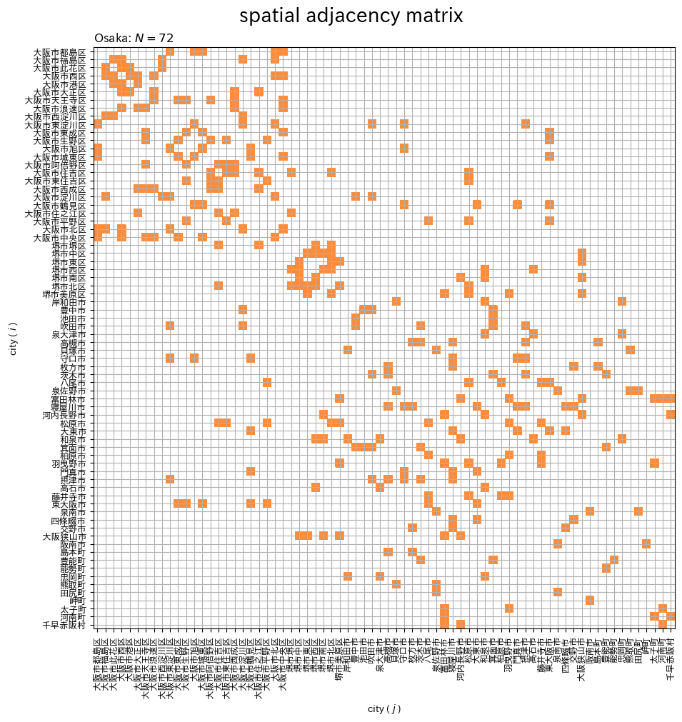
タイルの色は単色で指定できないので、グラデーションの範囲の引数 vmin, vmax を調整して、隣接する組み合わせ(値が1の要素)のタイルの色を設定します。
隣接しない組み合わせ(値が0の要素)はマスクしてタイルを色付けしません。
隣接する区域の組み合わせ( の要素)を色付けして示します。空間隣接行列は対称行列であるのを確認できます。
隣接区域のネットワーク図を作成します。
# 隣接ネットワークを作図
fig, ax = plt.subplots(nrows=1, ncols=1, constrained_layout=True,
                       figsize=(10, 10), dpi=100, facecolor='white')
gdf_district.boundary.plot(ax=ax, linewidth=0.5, edgecolor='black') # 行政区界
for j in range(N):
    # 隣接区域のインデックスを抽出
    adj_idx, = np.where(adj_mat[:, j] == 1)
    adj_idx = adj_idx[adj_idx > j] # 重複を除去
    for i in adj_idx:
        ax.plot([gdf_target.centers.x[j], gdf_target.centers.x[i]],
                [gdf_target.centers.y[j], gdf_target.centers.y[i]],
                color='C0') # 各区域-隣接区域
for x, y, label in zip(gdf_target.centers.x, gdf_target.centers.y, gdf_target.city2_label):
    ax.annotate(text=label, xy=(x-0.015, y-0.005), size=9) # 区域名
ax.set_xlabel('longitude')
ax.set_ylabel('latitude')
ax.set_title(f'Osaka: $N = {N}$', loc='left')
fig.suptitle('adjacency', fontsize=20)
ax.grid()
ax.set_aspect('equal', adjustable='box')
plt.show()

区域 j と隣接する区域の番号は、adj_mat[:, j] のうち値が 1 の要素インデックスです。
gdf_target の中心座標 centers 列から、隣接区域 j, i のx座標とy座標の値を取り出して、2点を線分で結びます。
隣接区域(値が1の組み合わせ)を線分で示します。
空間隣接行列と隣接ネットワークの対応をアニメーションで確認します。
作図コード(クリックで展開)
# 地区数を取得
N = len(gdf_target)

# 色の調整用
w_min, w_max = 0.0, 2.0

# 隣接区域以外を非表示化
adj_mat_masked = np.ma.masked_where(adj_mat==0, adj_mat)

# グラフオブジェクトを初期化
fig, axes = plt.subplots(nrows=1, ncols=2, constrained_layout=True,
                         figsize=(20, 10), width_ratios=[1, 1], dpi=100, facecolor='white')
fig.suptitle('spatial adjacency matrix', fontsize=20)

# 作図処理を定義
def update(n):

    # 前フレームのグラフを初期化
    [ax.cla() for ax in axes]

    # 隣接関係を格納
    tmp_adj_col = adj_mat[:, n].astype('float64') # 隣接関係を取得
    tmp_adj_col[tmp_adj_col == 0.0] = np.nan # 非隣接区域を非表示化
    gdf_target['adjacency'] = tmp_adj_col

    # 隣接ネットワークを作図
    ax = axes[0]
    gdf_district.boundary.plot(ax=ax, linewidth=0.5, edgecolor='black') # 行政区界
    gdf_target.plot(ax=ax, column='adjacency', cmap='Oranges', vmin=w_min, vmax=w_max) # 各区域の値
    for j in range(N):
        # 隣接区域のインデックスを抽出
        adj_idx, = np.where(adj_mat[:, j] == 1)
        adj_idx = adj_idx[adj_idx > j] # 重複を除去
        for i in adj_idx:
            ax.plot([gdf_target.centers.x[j], gdf_target.centers.x[i]],
                    [gdf_target.centers.y[j], gdf_target.centers.y[i]],
                    color='C0', linewidth=1.0) # 各区域-隣接区域
    # 隣接区域のインデックスを抽出
    adj_idx, = np.where(adj_mat[n] == 1)
    for i in adj_idx:
        ax.plot([gdf_target.centers.x[n], gdf_target.centers.x[i]],
                [gdf_target.centers.y[n], gdf_target.centers.y[i]],
                color='red', linewidth=2.5) # 対象区域-隣接区域
    for x, y, label in zip(gdf_target.centers.x, gdf_target.centers.y, gdf_target.city2_label):
        ax.annotate(text=label, xy=(x-0.015, y-0.005), size=9) # 区域名
    ax.set_xlabel('longitude')
    ax.set_ylabel('latitude')
    ax.set_title(f'Osaka: $N = {N}$', loc='left')
    ax.grid()
    ax.set_aspect('equal', adjustable='box')

    # 対象区域以外・隣接区域以外を非表示化
    target_mat_bool = np.tile(True, reps=adj_mat.shape)
    target_mat_bool[:, n] = False
    target_mat_masked = np.ma.masked_array(adj_mat_masked, target_mat_bool)

    # 空間隣接行列を作図
    ax = axes[1]
    ax.pcolor(adj_mat_masked, cmap='Oranges', vmin=w_min, vmax=w_max) # 全区域
    ax.pcolor(target_mat_masked, cmap='Oranges', vmin=w_min, vmax=w_max, color='red') # 対象区域の隣接区域
    ax.vlines(x=n+0.5, ymin=0, ymax=N, color='red', linestyle='dashed') # 対象区域
    ax.set_xticks(ticks=np.arange(N)+0.5)
    ax.set_xticklabels(labels=gdf_target.city2, size=9, rotation=90)
    ax.set_yticks(ticks=np.arange(N)+0.5)
    ax.set_yticklabels(labels=gdf_target.city2, size=9)
    ax.invert_yaxis() # 軸の反転
    ax.set_xlabel('city ( $j$ )')
    ax.set_ylabel('city ( $i$ )')
    ax.set_title(f'{gdf_target.city2[n]}: $\\sum_{{i=1}}^N w_{{ij}} = {np.sum(adj_mat[n])}$', loc='left') # 対象区域の隣接数
    ax.grid()
    ax.set_aspect('equal', adjustable='box')

# 動画を作成
ani = FuncAnimation(fig=fig, func=update, frames=N, interval=1000)

# 動画を書出
ani.save(
    filename='ch2_1_adjacency_matrix.mp4',
    progress_callback = lambda i, n: print(f'frame: {i} / {n}')
)
隣接区域のネットワーク図と空間隣接行列のヒートマップ上で、区域ごとに隣接区域を点や線で示します。隣接行列の列とネットワークが対応しているのを確認できます。
隣接行列の行和をデータフレームに格納します。
# 隣接区域数を格納
gdf_target['count'] = np.sum(adj_mat, axis=1)
gdf_target
出力(クリックで展開)
| city1 | city2 | d_code | geometry | centers | log_price | city2_label | count | |
|---|---|---|---|---|---|---|---|---|
| 0 | 大阪市 | 大阪市都島区 | 27102 | POLYGON ((135.51481 34.72057, 135.51489 34.720... | POINT (135.52721 34.71193) | 12.769969 | 都島区 | 5 |
| 1 | 大阪市 | 大阪市福島区 | 27103 | POLYGON ((135.46247 34.6874, 135.46253 34.6879... | POINT (135.47534 34.6939) | 13.214822 | 福島区 | 5 |
| 2 | 大阪市 | 大阪市此花区 | 27104 | MULTIPOLYGON (((135.36506 34.6325, 135.35885 3... | POINT (135.42012 34.668) | 12.191524 | 此花区 | 4 |
| 3 | 大阪市 | 大阪市西区 | 27106 | POLYGON ((135.46667 34.67284, 135.4642 34.6747... | POINT (135.48375 34.67776) | 13.746399 | 西区 | 7 |
| 4 | 大阪市 | 大阪市港区 | 27107 | MULTIPOLYGON (((135.43009 34.64977, 135.4301 3... | POINT (135.45084 34.66032) | 12.410058 | 港区 | 3 |
| ... | ... | ... | ... | ... | ... | ... | ... | ... |
| 67 | 泉南郡 | 田尻町 | 27362 | MULTIPOLYGON (((135.29259 34.40094, 135.29293 ... | POINT (135.25775 34.417) | 10.923984 | 田尻町 | 2 |
| 68 | 泉南郡 | 岬町 | 27366 | MULTIPOLYGON (((135.18163 34.34026, 135.18187 ... | POINT (135.15203 34.30321) | 9.918761 | 岬町 | 1 |
| 69 | 南河内郡 | 太子町 | 27381 | POLYGON ((135.66132 34.53314, 135.66139 34.532... | POINT (135.65269 34.51765) | 10.697891 | 太子町 | 3 |
| 70 | 南河内郡 | 河南町 | 27382 | MULTIPOLYGON (((135.64123 34.45932, 135.64105 ... | POINT (135.64897 34.48455) | 10.327751 | 河南町 | 3 |
| 71 | 南河内郡 | 千早赤阪村 | 27383 | POLYGON ((135.62578 34.47662, 135.62579 34.476... | POINT (135.64812 34.43844) | 10.122623 | 千早赤阪村 | 3 |
72 rows × 8 columns
区域ごとの隣接数(空間隣接行列の行和)を格納します(列和を使っても同じ結果になりますが、空間重み行列との対応からここでは行和を使います)。
隣接数のコロプレス図を作成します。
# 隣接ネットワークを作図
fig, ax = plt.subplots(nrows=1, ncols=1, constrained_layout=True,
                       figsize=(10, 10), dpi=100, facecolor='white')
gdf_district.boundary.plot(ax=ax, linewidth=0.5, edgecolor='white') # 行政区界
gdf_target.plot(ax=ax, column='count', cmap='jet', legend=True, legend_kwds={'label': 'count'}) # 隣接数
for i in range(len(adj_mat)):
    # 隣接区域のインデックスを抽出
    adj_idx, = np.where(adj_mat[i] == 1)
    adj_idx = adj_idx[adj_idx > i] # 重複を除去
    for j in adj_idx:
        ax.plot([gdf_target.centers.x[i], gdf_target.centers.x[j]],
                [gdf_target.centers.y[i], gdf_target.centers.y[j]],
                color='C0') # 各区域-隣接区域
for x, y, label in zip(gdf_target.centers.x, gdf_target.centers.y, gdf_target.city2_label):
    ax.annotate(text=label, xy=(x-0.015, y-0.005), size=9) # 区域名
ax.set_xlabel('longitude')
ax.set_ylabel('latitude')
ax.set_title(f'Osaka: $N = {len(gdf_target)}$', loc='left')
fig.suptitle('adjacency', fontsize=20)
ax.grid()
ax.set_aspect('equal', adjustable='box')
plt.show()

隣接数が少ないほど濃い青色、多いほど濃い赤色のグラデーションで区域ごとの隣接数を示しています。
この記事では、空間隣接行列を確認しました。次の記事では、空間重み行列を確認します。
参考文献
おわりに
私がとてもお世話になった先生の本です。本に載っていない図を作ったり、書いていないことを試したり、寄り道回り道しながらじっくりしっかり読んでいきます。
2章の内容ですが、このシリーズでは最初に投稿した記事です。1章の内容について追加でやってみると面白そうなことって何かあるでしょうか。思い付きませんでした。まだまだです。
2024年7月13日は、モーニング娘。の元リーダーの道重さゆみさんの35歳のお誕生日です!!!
おめでとうございます!今後もよろしくお願いします。
モーニング娘。時代のような表立った活動は控えめに見えますが、毎年のようにアルバムをリリースしライブをされていて、先月には(大手の)音楽サブスクが解禁されたので是非とも聴いてください。ライブ映像のサブスクもありますよ!
【次の内容】