はじめに

　『ベイズ推論による機械学習入門』(MLSシリーズ)の独学時のノートです。各種のモデルやアルゴリズムについて「数式・プログラム・図」を用いて解説します。
　本の補助として読んでください。

　この記事では、平均が未知の多次元ガウス分布に対するベイズ推論をPythonでスクラッチ実装します。

【前節の内容】

【他の節の内容】

【この節の内容】

3.4.1 多次元ガウス分布のベイズ推論の実装：平均が未知の場合

　多次元ガウスモデル(multivarate Gaussian model)に対するベイズ推論(Bayesian inference)を実装して、人工的に生成したデータを用いて、パラメータの学習と未知変数の予測を行う。この記事では、生成分布の平均パラメータ(mean parameter)が未知の場合を扱う。平均が未知の多次元ガウスモデルでは、尤度関数を多次元ガウス分布(multivariate Gaussian distribution・多変量正規分布・Normal distribution)、事前分布を多次元ガウス分布とする。この記事では、Pythonを利用して実装する。
　多次元ガウスモデルについては「3.4.0：多次元ガウスモデルの生成モデルの導出【緑ベイズ入門のノート】 - からっぽのしょこ」、ベイズ推論については「3.4.1：多次元ガウス分布のベイズ推論の導出：平均が未知の場合【緑ベイズ入門のノート】 - からっぽのしょこ」、Rを利用する場合は「【R】3.4.1：多次元ガウス分布のベイズ推論の実装：平均が未知の場合【緑ベイズ入門のノート】 - からっぽのしょこ」を参照のこと。

　利用するライブラリを読み込む。

# ライブラリを読込
import numpy as np
from scipy.stats import multivariate_normal
import matplotlib.pyplot as plt
import matplotlib.cm as cm
import matplotlib.patches as mpatches

ベイズ推論の実装

　まずは、平均が未知の多次元ガウス分布に対するベイズ推論における一連の処理を確認する。
　生成モデル(平均が未知の多次元ガウスモデル)を設定して、モデルに従うデータ(トイデータ)を生成する。続いて、生成した観測データを用いて、事後分布の計算(パラメータの推定)を行う。さらに、事後分布のパラメータ(または観測データ)を用いて、予測分布の計算(未観測データの予測)を行う。

生成分布の設定

　データの生成分布(真の分布・ガウス分布) $p(\mathbf{x}_n \mid \boldsymbol{\mu}_{\mathrm{truth}}, \boldsymbol{\Lambda}) = \mathcal{N}(\mathbf{x}_n \mid \boldsymbol{\mu}_{\mathrm{truth}}, \boldsymbol{\Lambda}^{-1})$ のパラメータ(真のパラメータ) $\boldsymbol{\mu}_{\mathrm{truth}}, \boldsymbol{\Lambda}$ を設定する。 $\boldsymbol{\Lambda}$ は既知とする。
　この例では、2次元のグラフで可視化するため、次元数を $D = 2$ とする。パラメータ推定の処理自体は次元数に関わらず行える。
　ガウス分布については「分布の作図」を参照のこと。

　生成分布のパラメータ $\boldsymbol{\mu}_{\mathrm{truth}}, \boldsymbol{\Lambda}$ を設定する。

# 次元数を設定
D = 2

# 真のパラメータを指定
mu_truth_d = np.array(
    [25.0, 50.0]
)
print(mu_truth_d)

# 既知のパラメータを指定
sigma2_dd = np.array(
    [[900.0, -100.0], 
     [-100.0, 400.0]]
)
print(sigma2_dd)

# 精度行列に変換
lambda_dd = np.linalg.inv(sigma2_dd)
print(lambda_dd)

[25. 50.]
[[ 900. -100.]
 [-100.  400.]]
[[0.00114286 0.00028571]
 [0.00028571 0.00257143]]

　ガウス分布の平均パラメータ(平均ベクトル・実数ベクトル) $\boldsymbol{\mu}$ 、分散パラメータ(分散共分散行列・正定値行列) $\boldsymbol{\Sigma}$ を指定して、精度パラメータ(精度行列) $\boldsymbol{\Lambda} = \boldsymbol{\Sigma}^{-1}$ を計算する。

$\displaystyle \boldsymbol{\mu} = \begin{bmatrix} \mu_1 \\ \mu_2 \end{bmatrix} ,\ \boldsymbol{\Sigma} = \begin{bmatrix} \sigma_1^2 & \sigma_{1,2} \\ \sigma_{2,1} & \sigma_2^2 \end{bmatrix}$

　 $\boldsymbol{\mu}_{\mathrm{truth}}$ がガウスモデルにおける真のパラメータであり、この値を求めるのがここでの目的(学習)である。

　生成分布の確率変数 $x_1, x_2$ の作図範囲を設定する。

# x軸の範囲を設定
k = 3
u = 5
x_0_size  = np.sqrt(sigma2_dd[0, 0]) # 基準値を指定
x_1_size  = np.sqrt(sigma2_dd[1, 1]) # 基準値を指定
x_0_size *= k # 定数倍
x_1_size *= k # 定数倍
#x_0_size  = max(x_0_size, *np.abs(x_nd[:, 0]-mu_truth_d[0])) # サンプルと比較
#x_1_size  = max(x_1_size, *np.abs(x_nd[:, 1]-mu_truth_d[1])) # サンプルと比較
x_0_size  = np.ceil(x_0_size /u)*u # u単位で切り上げ
x_1_size  = np.ceil(x_1_size /u)*u # u単位で切り上げ
x_0_min   = mu_truth_d[0] - x_0_size
x_0_max   = mu_truth_d[0] + x_0_size
x_1_min   = mu_truth_d[1] - x_1_size
x_1_max   = mu_truth_d[1] + x_1_size
print(x_0_min, x_0_max)
print(x_1_min, x_1_max)

# x軸の値を作成
x_0_vec = np.linspace(start=x_0_min, stop=x_0_max, num=251)
x_1_vec = np.linspace(start=x_1_min, stop=x_1_max, num=251)
print(x_0_vec[:5])
print(x_1_vec[:5])

-65.0 115.0
-10.0 110.0
[-65.   -64.28 -63.56 -62.84 -62.12]
[-10.    -9.52  -9.04  -8.56  -8.08]

　この例では、指定したパラメータ(または生成したデータ)を使って、範囲を設定している。

　格子点 $(x_1, x_2)$ を作成する。

# 格子点を作成
x_0_grid, x_1_grid = np.meshgrid(x_0_vec, x_1_vec)
print(x_0_grid[:5, :5])
print(x_1_grid[:5, :5])

# 格子点の座標を整形
x_arr  = np.stack([x_0_grid.flatten(), x_1_grid.flatten()], axis=1)
x_dims = x_0_grid.shape
print(x_arr[:5])
print(x_dims)

[[-65.   -64.28 -63.56 -62.84 -62.12]
 [-65.   -64.28 -63.56 -62.84 -62.12]
 [-65.   -64.28 -63.56 -62.84 -62.12]
 [-65.   -64.28 -63.56 -62.84 -62.12]
 [-65.   -64.28 -63.56 -62.84 -62.12]]
[[-10.   -10.   -10.   -10.   -10.  ]
 [ -9.52  -9.52  -9.52  -9.52  -9.52]
 [ -9.04  -9.04  -9.04  -9.04  -9.04]
 [ -8.56  -8.56  -8.56  -8.56  -8.56]
 [ -8.08  -8.08  -8.08  -8.08  -8.08]]
[[-65.   -10.  ]
 [-64.28 -10.  ]
 [-63.56 -10.  ]
 [-62.84 -10.  ]
 [-62.12 -10.  ]]
(251, 251)

　 $x_1, x_2$ の値の全ての組み合わせ(格子状の点)を np.meshgrid() で作成して、複製された軸ごとの値(作図用の配列)を x_0_grid, x_1_grid、2つの軸の値をまとめた座標(計算用の配列)を x_arr とする。

　生成分布の確率密度を計算する。

# 生成分布の確率密度を計算:式(2.72)
model_dens_grid = multivariate_normal.pdf(
    x=x_arr, mean=mu_truth_d, cov=sigma2_dd
).reshape(x_dims)
print(model_dens_grid.flatten()[:5])

[5.48789388e-09 5.98136214e-09 6.51534158e-09 7.09278802e-09
 7.71683956e-09]

　 $\mathbf{x} = (x_1, x_2)^{\top}$ の点ごとに、ガウス分布に従う確率密度 $\mathcal{N}(\mathbf{x} \mid \boldsymbol{\mu}_{\mathrm{truth}}, \boldsymbol{\Lambda}^{-1})$ を計算する。
　多次元ガウス分布の確率密度関数 sp.stats.multivariate\_normal.pdf() の確率変数の引数 x に $\mathbf{x}$ 、平均ベクトルの引数 mean に $\boldsymbol{\mu}_{\mathrm{truth}}$ 、分散共分散行列の引数 cov に $\boldsymbol{\Sigma} = \boldsymbol{\Lambda}^{-1}$ を指定する。

　生成分布のグラフを作成する。

# p(x)軸の範囲を設定
u = 0.00005
dens_min       = 0.0
model_dens_max = model_dens_grid.max()
model_dens_max = np.ceil(model_dens_max /u)*u # u単位で切り上げ

# 生成分布のラベルを作成
tmp_lmd_0_str = ', '.join([f'{lmd:.5f}' for lmd in lambda_dd[0, :]])
tmp_lmd_1_str = ', '.join([f'{lmd:.5f}' for lmd in lambda_dd[1, :]])
model_param_lbl  = f'$\\mu_{{truth}} = \\binom{{{mu_truth_d[0]:.2f}}}{{{mu_truth_d[1]:.2f}}}, '
model_param_lbl += f'\\Lambda = \\binom{{{tmp_lmd_0_str}}}{{{tmp_lmd_1_str}}}$'

# 生成分布を作図
fig, ax = plt.subplots(
    figsize=(9, 6), dpi=100, facecolor='white', 
    constrained_layout=True
)
fig.suptitle('multivariate Gaussian distribution', fontsize=20)

cs = ax.contourf(
    x_0_grid, x_1_grid, model_dens_grid, 
    cmap='YlOrRd_r', vmin=dens_min, vmax=model_dens_max, 
    alpha=0.5, 
    zorder=10
) # 真の分布
dummy = plt.Line2D(
    [], [], 
    color='red', linewidth=1.0, linestyle='--', 
    label='true model'
) # (凡例表示用のダミー)

ax.set_xlabel('$x_1$')
ax.set_ylabel('$x_2$')
ax.set_title(model_param_lbl, loc='left') # パラメータラベル
fig.colorbar(cs, ax=ax, shrink=1.0, label='density')
ax.legend(handles=[dummy], prop={'size': 8})
ax.grid(zorder=0)

plt.show()

# 生成分布を作図
fig, ax = plt.subplots(
    figsize=(9, 6), dpi=100, facecolor='white', 
    constrained_layout=True, subplot_kw={'projection': '3d'}
)
fig.suptitle('multivariate Gaussian distribution', fontsize=20)

ax.contour(
    X=x_0_grid, Y=x_1_grid, Z=model_dens_grid, offset=0.0, 
    cmap='YlOrRd_r', vmin=dens_min, vmax=model_dens_max, 
    linewidths=1.0, linestyles=':', 
    zorder=10
) # 真の分布
ax.contour(
    X=x_0_grid, Y=x_1_grid, Z=model_dens_grid, 
    cmap='YlOrRd_r', vmin=dens_min, vmax=model_dens_max, 
    linewidths=1.0, linestyles='-', 
    zorder=11
) # 真の分布
ax.plot_surface(
    X=x_0_grid, Y=x_1_grid, Z=model_dens_grid, 
    cmap='YlOrRd_r', vmin=dens_min, vmax=model_dens_max, 
    alpha=0.8, 
    label='true model', 
    zorder=12
) # 真の分布

ax.set_xlabel('$x_1$')
ax.set_ylabel('$x_2$')
ax.set_zlabel('density')
ax.set_title(model_param_lbl, loc='left') # パラメータラベル
ax.legend(prop={'size': 8})

plt.show()

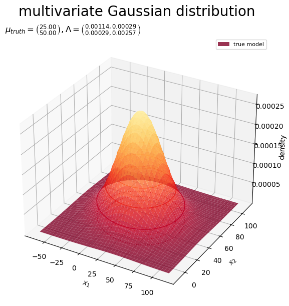
　真の分布(ガウス分布)を等高線や曲面(グラデーション)で示す。

　真のパラメータ $\boldsymbol{\mu}_{\mathrm{truth}}$ を求めることは、真の分布 $\mathcal{N}(\mathbf{x}_n \mid \boldsymbol{\mu}_{\mathrm{truth}}, \boldsymbol{\Lambda}^{-1})$ を求めることを意味する。

データの生成

　設定した生成分布(ガウス分布) $p(\mathbf{x}_n \mid \boldsymbol{\mu}_{\mathrm{truth}}, \boldsymbol{\Lambda}) = \mathcal{N}(\mathbf{x}_n \mid \boldsymbol{\mu}_{\mathrm{truth}}, \boldsymbol{\Lambda}^{-1})$ に従うデータ(観測データ) $\mathbf{X}$ を作成する。
　ガウスモデルのデータ生成については「乱数の生成」を参照のこと。

　生成分布からデータ $\mathbf{X}$ を生成する。

# データ数を指定
N = 300

# 観測データを生成
x_nd = np.random.multivariate_normal(
    mean=mu_truth_d, cov=sigma2_dd, size=N
)
print(x_nd[:5])

[[40.51875715 34.98099892]
 [ 9.10105428 40.67775906]
 [ 0.10057259 31.9014864 ]
 [78.76090384 75.45144699]
 [30.58235046 72.0455999 ]]

　データ数 $N$ を指定して、多次元ガウス分布に従う乱数 $\mathbf{X} = {\mathbf{x}_1, \cdots, \mathbf{x}_N}$ 、 $\mathbf{x}_n = (x_{n,1}, x_{n,2})^{\top}$ を生成する。
　多次元ガウス分布の乱数生成関数 np.random.multivariate_normal() の平均ベクトルの引数 mean に $\boldsymbol{\mu}_{\mathrm{truth}}$ 、分散共分散行列の引数 cov に $\boldsymbol{\Sigma} = \boldsymbol{\Lambda}^{-1}$ 、サンプルサイズの引数 size に $N$ を指定する。

　観測データ $\mathbf{X}$ を集計する。

# 階級数を指定
class_0_num = 46
class_1_num = 31

# 境界数を設定
bin_0_num = class_0_num + 1
bin_1_num = class_1_num + 1

# 階級幅を計算
bin_0_size = (x_0_max - x_0_min) / (class_0_num-1)
bin_1_size = (x_1_max - x_1_min) / (class_1_num-1)
print(bin_0_size)
print(bin_1_size)

# 境界値の範囲を設定
bin_0_min = x_0_min - 0.5*bin_0_size
bin_0_max = x_0_max + 0.5*bin_0_size
bin_1_min = x_1_min - 0.5*bin_1_size
bin_1_max = x_1_max + 0.5*bin_1_size

# 度数を集計
obs_freq_grid, bin_0_vec, bin_1_vec = np.histogram2d(
    x=x_nd[:, 0], y=x_nd[:, 1], 
    bins=(class_0_num, class_1_num), 
    range=[(bin_0_min, bin_0_max), (bin_1_min, bin_1_max)]
)
print(bin_0_vec[:5])
print(bin_1_vec[:5])
print(obs_freq_grid[:5, :5])

# 密度を計算
obs_dens_grid = obs_freq_grid / (bin_0_size * bin_1_size * N)
print(obs_dens_grid[:5, :5])

# 階級値を作成
center_0_vec = bin_0_vec[:-1] + 0.5*bin_0_size
center_1_vec = bin_1_vec[:-1] + 0.5*bin_1_size
print(center_0_vec[:5])
print(center_1_vec[:5])

4.0
4.0
[-67. -63. -59. -55. -51.]
[-12.  -8.  -4.   0.   4.]
[[0. 0. 1. 0. 0.]
 [0. 0. 0. 0. 0.]
 [0. 0. 0. 0. 0.]
 [0. 0. 0. 0. 0.]
 [0. 0. 0. 0. 0.]]
[[0.         0.         0.00020833 0.         0.        ]
 [0.         0.         0.         0.         0.        ]
 [0.         0.         0.         0.         0.        ]
 [0.         0.         0.         0.         0.        ]
 [0.         0.         0.         0.         0.        ]]
[-65. -61. -57. -53. -49.]
[-10.  -6.  -2.   2.   6.]

　階級数を指定して、階級幅 $w_1, w_2$ を設定する。
　 $x_1, x_2$ の範囲で階級値を作成して、観測データ x_nd に含まれる要素数をカウントして、度数 $N_{x_1,x_2}$ と密度 $\frac{N_{x_1,x_2}}{w_1 w_2 N}$ を求める。

　観測データ $\mathbf{X}$ のグラフを作成する。

# 観測データのラベルを作成
tmp_lmd_0_str = ', '.join([f'{lmd:.5f}' for lmd in lambda_dd[0, :]])
tmp_lmd_1_str = ', '.join([f'{lmd:.5f}' for lmd in lambda_dd[1, :]])
obs_param_lbl  = f'$N = {N}, '
obs_param_lbl += f'\\mu_{{truth}} = \\binom{{{mu_truth_d[0]:.2f}}}{{{mu_truth_d[1]:.2f}}}, '
obs_param_lbl += f'\\Lambda = \\binom{{{tmp_lmd_0_str}}}{{{tmp_lmd_1_str}}}$'

# 観測データを作図
fig, ax = plt.subplots(
    figsize=(9, 6), dpi=100, facecolor='white', 
    constrained_layout=True
)
fig.suptitle('multivariate Gaussian distribution', fontsize=20)

pcm = ax.pcolormesh(
    center_0_vec, center_1_vec, obs_dens_grid.T, 
    shading='nearest', 
    cmap='YlOrRd_r', #vmin=dens_min, vmax=model_dens_max, # (軸目盛の共通化用) ## (Nが不十分な場合はスケールを統一しない方が意図に近い図になる)
    alpha=0.5, 
    zorder=10
) # 観測データ
cs = ax.contour(
    x_0_grid, x_1_grid, model_dens_grid, 
    cmap='YlOrRd_r', vmin=dens_min, vmax=model_dens_max, # (軸目盛の共通化用)
    linewidths=1.0, linestyles='--', 
    zorder=11
) # 生成分布
model_dummy = plt.Line2D(
    [], [], 
    color='red', linewidth=1.0, linestyle='--', 
    label='true model'
) # (凡例表示用のダミー)
obs_dummy = mpatches.Patch(
    color='hotpink', 
    label='observation data'
) # (凡例表示用のダミー)

ax.set_xlabel('$x_1$')
ax.set_ylabel('$x_2$')
ax.set_title(obs_param_lbl, loc='left') # パラメータラベル
fig.colorbar(cs, ax=ax, shrink=1.0, label='density')
fig.colorbar(pcm, ax=ax, shrink=1.0, label='density') ## (スケールが異なる場合はそれぞれのカラーバーを表示する)
ax.legend(handles=[model_dummy, obs_dummy], prop={'size': 8})
ax.grid(zorder=0)

plt.show()

# 作図用の座標を作成
bin_0_grid, bin_1_grid = np.meshgrid(bin_0_vec[:-1], bin_1_vec[:-1])

# 観測データを作図
fig, ax = plt.subplots(
    figsize=(9, 6), dpi=100, facecolor='white', 
    constrained_layout=True, subplot_kw={'projection': '3d'}
)
fig.suptitle('multivariate Gaussian distribution', fontsize=20)

ax.contour(
    X=x_0_grid, Y=x_1_grid, Z=model_dens_grid, offset=0.0, 
    cmap='YlOrRd_r', vmin=dens_min, vmax=model_dens_max, 
    linewidths=1.0, linestyles=':', 
    zorder=10
) # 生成分布
ax.plot_wireframe(
    X=x_0_grid, Y=x_1_grid, Z=model_dens_grid, 
    color='red', linewidth=0.5, linestyle='--', 
    label='true model', 
    zorder=12
) # 生成分布
ax.bar3d(
    x=bin_0_grid.flatten(), y=bin_1_grid.flatten(), z=0.0, 
    dx=bin_0_size, dy=bin_1_size, dz=obs_dens_grid.flatten(), 
    color=(1.0, 1.0, 1.0, 0.05), 
    edgecolor='hotpink', linewidths=0.1, 
    label='observation data', 
    zorder=11
) # 観測データ

ax.set_xlabel('$x_1$')
ax.set_ylabel('$x_2$')
ax.set_zlabel('density')
ax.set_title(obs_param_lbl, loc='left') # パラメータラベル
ax.legend(prop={'size': 8})

#ax.set_zlim(zmin=dens_min, zmax=model_dens_max) # 表示範囲
ax.view_init(elev=0, azim=-60) # 表示角度
plt.show()

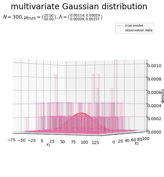
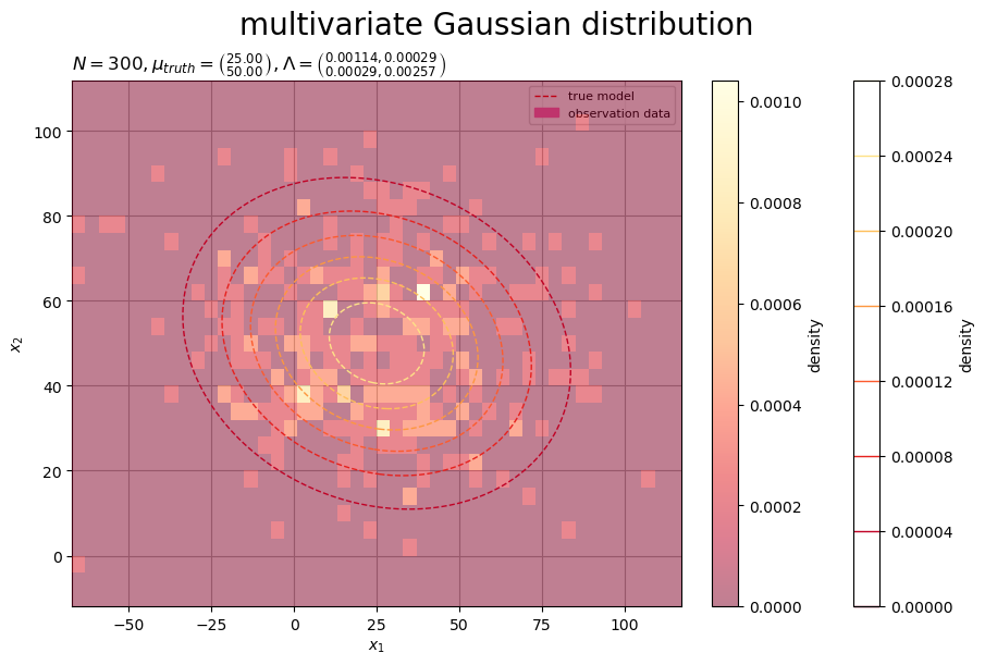
　 $\mathbf{x}$ の値ごとの確率密度(生成分布)を等高線や曲面(赤色・破線)、観測データ $\mathbf{X}$ の度数 $N_{x_1,x_2}$ (密度 $\frac{N_{x_1,x_2}}{w_1 w_2 N}$ )をヒートマップ(グラデーション)や3D棒グラフ(桃色)で示す。

　データ数 $N$ が十分に大きいと、観測データ $\mathbf{X}$ のヒートマップの形状が生成分布 $\mathcal{N}(\mathbf{x}_n \mid \boldsymbol{\mu}_{\mathrm{truth}}, \boldsymbol{\Lambda}^{-1})$ に近付く。

事前分布の設定

　パラメータ $\boldsymbol{\mu}$ の事前分布(ガウス分布) $p(\boldsymbol{\mu} \mid \mathbf{m}, \boldsymbol{\Lambda}_{\mu}) = \mathcal{N}(\boldsymbol{\mu} \mid \mathbf{m}, \boldsymbol{\Lambda}_{\mu}^{-1})$ のパラメータ(超パラメータ) $\mathbf{m}, \boldsymbol{\Lambda}$ を設定する。

　事前分布のパラメータ $\mathbf{m}, \boldsymbol{\Lambda}_{\mu}$ を設定する。

# 事前分布のパラメータを指定
m_d          = np.tile(0.0, reps=D)
sigma2_mu_dd = np.identity(D) * 100**2
print(m_d)
print(sigma2_mu_dd)

# 精度行列に変換
lambda_mu_dd = np.linalg.inv(sigma2_mu_dd)
print(lambda_mu_dd)

[0. 0.]
[[10000.     0.]
 [    0. 10000.]]
[[0.0001 0.    ]
 [0.     0.0001]]

　ガウス分布の平均パラメータ(平均パラメータ・実数ベクトル) $\mathbf{m}$ 、分散パラメータ(分散共分散行列・正定値行列) $\boldsymbol{\Sigma}_{\mu}$ を指定して、精度パラメータ(精度行列) $\boldsymbol{\Lambda}_{\mu} = \boldsymbol{\Sigma}_{\mu}^{-1}$ を計算する。

$\displaystyle \mathbf{m} = \begin{bmatrix} m_1 \\ m_2 \end{bmatrix} ,\ \boldsymbol{\Sigma}_{\mu} = \begin{bmatrix} \sigma_{\mu,1}^2 & \sigma_{\mu,1,2} \\ \sigma_{\mu,2,1} & \sigma_{\mu,2}^2 \end{bmatrix}$

　事前分布の確率変数 $\mu_1, \mu_2$ の作図範囲を設定する。

# μ軸の範囲を設定
mu_0_min, mu_0_max = x_0_min, x_0_max
mu_1_min, mu_1_max = x_1_min, x_1_max
print(mu_0_min, mu_0_max)
print(mu_1_min, mu_1_max)

# μ軸の値を作成
mu_0_vec = np.linspace(start=mu_0_min, stop=mu_0_max, num=251)
mu_1_vec = np.linspace(start=mu_1_min, stop=mu_1_max, num=251)
print(mu_0_vec[:5])
print(mu_1_vec[:5])

-65.0 115.0
-10.0 110.0
[-65.   -64.28 -63.56 -62.84 -62.12]
[-10.    -9.52  -9.04  -8.56  -8.08]

　この例では、生成分布の確率変数 $x_1, x_2$ の範囲を使っている。

　格子点 $(\mu_1, \mu_2)$ を作成する。

# 格子点を作成
mu_0_grid, mu_1_grid = np.meshgrid(mu_0_vec, mu_1_vec)
print(mu_0_grid[:5, :5])
print(mu_1_grid[:5, :5])

# 格子点の座標を作成
mu_arr  = np.stack([mu_0_grid.flatten(), mu_1_grid.flatten()], axis=1)
mu_dims = mu_0_grid.shape
print(mu_arr[:5])
print(mu_dims)

[[-65.   -64.28 -63.56 -62.84 -62.12]
 [-65.   -64.28 -63.56 -62.84 -62.12]
 [-65.   -64.28 -63.56 -62.84 -62.12]
 [-65.   -64.28 -63.56 -62.84 -62.12]
 [-65.   -64.28 -63.56 -62.84 -62.12]]
[[-10.   -10.   -10.   -10.   -10.  ]
 [ -9.52  -9.52  -9.52  -9.52  -9.52]
 [ -9.04  -9.04  -9.04  -9.04  -9.04]
 [ -8.56  -8.56  -8.56  -8.56  -8.56]
 [ -8.08  -8.08  -8.08  -8.08  -8.08]]
[[-65.   -10.  ]
 [-64.28 -10.  ]
 [-63.56 -10.  ]
 [-62.84 -10.  ]
 [-62.12 -10.  ]]
(251, 251)

　 $\mu_1, \mu_2$ の値の全ての組み合わせ(格子状の点)を np.meshgrid() で作成して、複製された軸ごとの値(作図用の配列)を mu_0_grid, mu_1_grid、2つの軸の値をまとめた座標(計算用の配列)を mu_arr とする。

　事前分布の確率密度を計算する。

# 事前分布の確率密度を計算:式(2.72)
prior_dens_grid = multivariate_normal.pdf(
    x=mu_arr, mean=m_d, cov=sigma2_mu_dd
).reshape(mu_dims)
print(prior_dens_grid.flatten()[:5])

[1.28204701e-05 1.28802767e-05 1.29396914e-05 1.29987063e-05
 1.30573135e-05]

　 $\boldsymbol{\mu} = (\mu_1, \mu_2)^{\top}$ の点ごとに、ガウス分布に従う確率密度 $\mathcal{N}(\boldsymbol{\mu} \mid \mathbf{m}, \boldsymbol{\Lambda}_{\mu}^{-1})$ を計算する。
　多次元ガウス分布の確率密度関数 sp.stats.multivariate_normal.pdf() の確率変数の引数 x に $\boldsymbol{\mu}$ 、平均ベクトルの引数 mean に $\mathbf{m}$ 、分散共分散行列の引数 cov に $\boldsymbol{\Sigma}_{\mu} = \boldsymbol{\Lambda}_{\mu}^{-1}$ を指定する。

　事前分布のグラフを作成する。

# 事前分布のラベルを作成
tmp_lmd_0_str = ', '.join([f'{lmd:.5f}' for lmd in lambda_mu_dd[0, :]])
tmp_lmd_1_str = ', '.join([f'{lmd:.5f}' for lmd in lambda_mu_dd[1, :]])
prior_param_lbl  = f'$\\mu_{{truth}} = \\binom{{{mu_truth_d[0]:.2f}}}{{{mu_truth_d[1]:.2f}}}, '
prior_param_lbl += f'm = \\binom{{{m_d[0]:.2f}}}{{{m_d[1]:.2f}}}, '
prior_param_lbl += f'\\Lambda_{{\\mu}} = \\binom{{{tmp_lmd_0_str}}}{{{tmp_lmd_1_str}}}$'

# 事前分布を作図
fig, ax = plt.subplots(
    figsize=(9, 6), dpi=100, facecolor='white', 
    constrained_layout=True
)
fig.suptitle('multivariate Gaussian distribution', fontsize=20)
ax2x = ax.twiny() # 第2軸の設定用
ax2y = ax.twinx() # 第2軸の設定用

cs = ax.contourf(
    mu_0_grid, mu_1_grid, prior_dens_grid, 
    cmap='viridis', alpha=0.5, 
    zorder=10
) # 事前分布
ax.plot(
    [[mu_truth_d[0], mu_0_min], [mu_truth_d[0], mu_0_max]], 
    [[mu_1_min, mu_truth_d[1]], [mu_1_max, mu_truth_d[1]]], 
    color='red', linewidth=1.0, linestyle='--', 
    label=['true parameter', None], 
    zorder=11
) # 真のパラメータ
ax.plot(
    [], [], 
    color='purple', linewidth=1.0, 
    label='prior distribution'
) # (凡例表示用のダミー)

ax2x.set_xticks(ticks=[mu_truth_d[0]], labels=['$\\mu_1^{truth}$']) # パラメータラベル
ax2y.set_yticks(ticks=[mu_truth_d[1]], labels=['$\\mu_2^{truth}$']) # パラメータラベル
ax.set_xlabel('$\\mu_1$')
ax.set_ylabel('$\\mu_2$')
ax.set_title(prior_param_lbl, loc='left') # パラメータラベル
fig.colorbar(cs, ax=ax, shrink=1.0, label='density')
ax.legend(prop={'size': 8})
ax.grid(zorder=0)
ax.set_xlim(xmin=mu_0_min, xmax=mu_0_max)   # (目盛の共通化用)
ax.set_ylim(ymin=mu_1_min, ymax=mu_1_max)   # (目盛の共通化用)
ax2x.set_xlim(xmin=mu_0_min, xmax=mu_0_max) # (目盛の共通化用)
ax2y.set_ylim(ymin=mu_1_min, ymax=mu_1_max) # (目盛の共通化用)

plt.show()

# 事前分布を作図
fig, ax = plt.subplots(
    figsize=(9, 6), dpi=100, facecolor='white', 
    constrained_layout=True, subplot_kw={'projection': '3d'}
)
fig.suptitle('multivariate Gaussian distribution', fontsize=20)

ax.plot(
    [mu_truth_d[0]]*2+[np.nan]+[mu_0_min, mu_0_max], 
    [mu_1_min, mu_1_max]+[np.nan]+[mu_truth_d[1]]*2, 
    [0.0, 0.0, np.nan, 0.0, 0.0], 
    color='red', linewidth=1.0, linestyle='--', 
    label='true parameter', 
    zorder=10
) # 真のパラメータ
ax.contour(
    X=mu_0_grid, Y=mu_1_grid, Z=prior_dens_grid, offset=0.0, 
    cmap='viridis', linewidths=1.0, linestyles=':', 
    zorder=11
) # 事前分布
ax.contour(
    X=mu_0_grid, Y=mu_1_grid, Z=prior_dens_grid, 
    cmap='viridis', linewidths=1.0, linestyles='-', 
    zorder=12
) # 事前分布
ax.plot_surface(
    X=mu_0_grid, Y=mu_1_grid, Z=prior_dens_grid, 
    cmap='viridis', alpha=0.8, 
    label='prior distribution', 
    zorder=13
) # 事前分布

ax.set_xlabel('$\\mu_1$')
ax.set_ylabel('$\\mu_2$')
ax.set_zlabel('density')
ax.set_title(prior_param_lbl, loc='left') # パラメータラベル
ax.legend(prop={'size': 8})

plt.show()

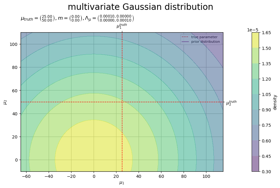
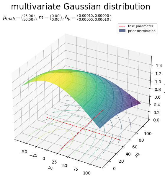
　真のパラメータを直線(赤色・破線)、事前分布(ガウス分布)を等高線や曲面(グラデーション)で示す。

　真のパラメータ(真の分布のパラメータ) $\boldsymbol{\mu}_{\mathrm{truth}}$ と、パラメータ $\boldsymbol{\mu}$ の事前分布 $\mathcal{N}(\boldsymbol{\mu} \mid \mathbf{m}, \boldsymbol{\Lambda}_{\mu})$ の位置関係を図で確認する。

事後分布の計算

　観測データ $\mathbf{X}$ から、パラメータ $\boldsymbol{\mu}$ の事後分布(ガウス分布) $p(\boldsymbol{\mu} \mid \mathbf{X}, \mathbf{m}, \boldsymbol{\Lambda}_{\mu}) = \mathcal{N}(\boldsymbol{\mu} \mid \hat{\mathbf{m}}, \hat{\boldsymbol{\Lambda}}_{\mu}^{-1})$ のパラメータ(超パラメータ) $\hat{\mathbf{m}}, \hat{\boldsymbol{\Lambda}}_{\mu}$ を求める(真のパラメータ $\boldsymbol{\mu}_{\mathrm{truth}}$ を分布推定する)。

　事後分布のパラメータ $\hat{\mathbf{m}}, \hat{\boldsymbol{\Lambda}}_{\mu}$ を計算する。

# 事後分布のパラメータを計算:式(3.102, 3.103)
lambda_mu_hat_dd = N * lambda_dd + lambda_mu_dd
m_hat_d          = np.linalg.inv(lambda_mu_hat_dd) @ (lambda_dd @ np.sum(x_nd, axis=0) + lambda_mu_dd @ m_d)
print(m_hat_d)
print(lambda_mu_hat_dd)

[24.25450664 49.43703419]
[[0.34295714 0.08571429]
 [0.08571429 0.77152857]]

　事後分布のパラメータは、次の式で計算できる。

$\displaystyle \begin{align} \hat{\mathbf{m}} &= \hat{\boldsymbol{\Lambda}}_{\mu}^{-1} \left( \boldsymbol{\Lambda} \sum_{n=1}^N \mathbf{x}_n + \boldsymbol{\Lambda}_{\mu} \mathbf{m} \right) \tag{3.103}\\ \hat{\boldsymbol{\Lambda}}_{\mu} &= N \boldsymbol{\Lambda} + \boldsymbol{\Lambda}_{\mu} \tag{3.102} \end{align}$

　事後分布の確率密度を計算する。

# 事後分布の確率密度を計算:式(2.72)
posterior_dens_grid = multivariate_normal.pdf(
    x=mu_arr, mean=m_hat_d, cov=np.linalg.inv(lambda_mu_hat_dd)
).reshape(mu_dims)
print(posterior_dens_grid.flatten()[:5])

[0. 0. 0. 0. 0.]

　事前分布のときと同様にして、ガウス分布に従う確率密度 $\mathcal{N}(\boldsymbol{\mu} \mid \hat{\mathbf{m}}, \hat{\boldsymbol{\Lambda}}_{\mu})$ を計算する。

　事後分布のグラフを作成する。

# 事後分布のラベルを作成
tmp_lmd_0_str = ', '.join([f'{lmd:.5f}' for lmd in lambda_mu_hat_dd[0, :]])
tmp_lmd_1_str = ', '.join([f'{lmd:.5f}' for lmd in lambda_mu_hat_dd[1, :]])
posterior_param_lbl  = f'$N = {N}, '
posterior_param_lbl += f'\\mu_{{truth}} = \\binom{{{mu_truth_d[0]:.2f}}}{{{mu_truth_d[1]:.2f}}}, '
posterior_param_lbl += f'\\hat{{m}} = \\binom{{{m_hat_d[0]:.2f}}}{{{m_hat_d[1]:.2f}}}, '
posterior_param_lbl += f'\\hat{{\\Lambda}}_{{\\mu}} = \\binom{{{tmp_lmd_0_str}}}{{{tmp_lmd_1_str}}}$'

# 事後分布を作図
fig, ax = plt.subplots(
    figsize=(9, 6), dpi=100, facecolor='white', 
    constrained_layout=True
)
fig.suptitle('multivariate Gaussian distribution', fontsize=20)
ax2x = ax.twiny() # 第2軸の設定用
ax2y = ax.twinx() # 第2軸の設定用

cs = ax.contourf(
    mu_0_grid, mu_1_grid, posterior_dens_grid, 
    cmap='viridis', alpha=0.5, 
    zorder=10
) # 事後分布
ax.plot(
    [[mu_truth_d[0], mu_0_min], [mu_truth_d[0], mu_0_max]], 
    [[mu_1_min, mu_truth_d[1]], [mu_1_max, mu_truth_d[1]]], 
    color='red', linewidth=1.0, linestyle='--', 
    label=['true parameter', None], 
    zorder=11
) # 真のパラメータ
ax.plot(
    [], [], 
    color='purple', linewidth=1.0, 
    label='posterior distribution'
) # (凡例表示用のダミー)

ax2x.set_xticks(ticks=[mu_truth_d[0]], labels=['$\\mu_1^{truth}$']) # パラメータラベル
ax2y.set_yticks(ticks=[mu_truth_d[1]], labels=['$\\mu_2^{truth}$']) # パラメータラベル
ax.set_xlabel('$\\mu_1$')
ax.set_ylabel('$\\mu_2$')
ax.set_title(posterior_param_lbl, loc='left') # パラメータラベル
fig.colorbar(cs, ax=ax, shrink=1.0, label='density')
ax.legend(prop={'size': 8})
ax.grid(zorder=0)
ax.set_xlim(xmin=mu_0_min, xmax=mu_0_max)   # (目盛の共通化用)
ax.set_ylim(ymin=mu_1_min, ymax=mu_1_max)   # (目盛の共通化用)
ax2x.set_xlim(xmin=mu_0_min, xmax=mu_0_max) # (目盛の共通化用)
ax2y.set_ylim(ymin=mu_1_min, ymax=mu_1_max) # (目盛の共通化用)

plt.show()

# 事後分布を作図
fig, ax = plt.subplots(
    figsize=(9, 6), dpi=100, facecolor='white', 
    constrained_layout=True, subplot_kw={'projection': '3d'}
)
fig.suptitle('multivariate Gaussian distribution', fontsize=20)

ax.plot(
    [mu_truth_d[0]]*2+[np.nan]+[mu_0_min, mu_0_max], 
    [mu_1_min, mu_1_max]+[np.nan]+[mu_truth_d[1]]*2, 
    [0.0, 0.0, np.nan, 0.0, 0.0], 
    color='red', linewidth=1.0, linestyle='--', 
    label='true parameter', 
    zorder=10
) # 真のパラメータ
ax.contour(
    X=mu_0_grid, Y=mu_1_grid, Z=posterior_dens_grid, offset=0.0, 
    cmap='viridis', linewidths=1.0, linestyles=':', 
    zorder=11
) # 事後分布
ax.contour(
    X=mu_0_grid, Y=mu_1_grid, Z=posterior_dens_grid, 
    cmap='viridis', linewidths=1.0, linestyles='-', 
    zorder=12
) # 事後分布
ax.plot_surface(
    X=mu_0_grid, Y=mu_1_grid, Z=posterior_dens_grid, 
    cmap='viridis', alpha=0.8, 
    label='posterior distribution', 
    zorder=13
) # 事後分布

ax.set_xlabel('$\\mu_1$')
ax.set_ylabel('$\\mu_2$')
ax.set_zlabel('density')
ax.set_title(posterior_param_lbl, loc='left') # パラメータラベル
ax.legend(prop={'size': 8})

plt.show()

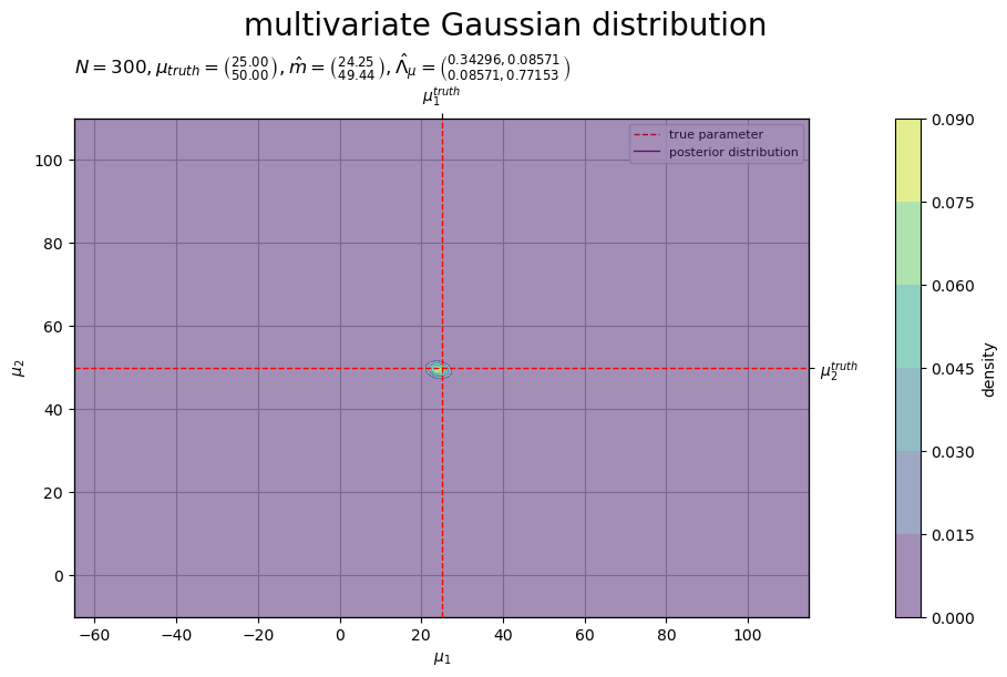
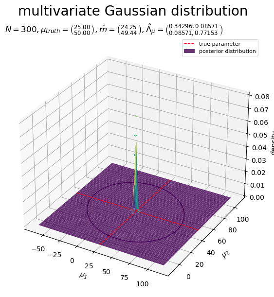
　真のパラメータを直線(赤色・破線)、事後分布(ガウス分布)を等高線や曲面(グラデーション)で示す。

　データ数 $N$ が十分に大きいと、パラメータ $\boldsymbol{\mu}$ の事後分布 $\mathcal{N}(\boldsymbol{\mu} \mid \hat{\mathbf{m}}, \hat{\boldsymbol{\Lambda}}_{\mu}^{-1})$ のピークが真のパラメータ $\boldsymbol{\mu}_{\mathrm{truth}}$ に近付く。

予測分布の計算

　観測データ $\mathbf{X}$ から、未観測のデータ $\mathbf{x}_{*}$ の予測分布(ガウス分布) $p(\mathbf{x}_{*} \mid \mathbf{X}, \mathbf{m}, \boldsymbol{\Lambda}_{\mu}) = \mathcal{N}(\mathbf{x}_{*} \mid \hat{\boldsymbol{\mu}}_{*}, \hat{\boldsymbol{\Lambda}}_{*}^{-1})$ を求める。

　予測分布のパラメータ $\hat{\boldsymbol{\mu}}_{*}, \hat{\boldsymbol{\Lambda}}_{*}$ を計算する。

# 予測分布のパラメータを計算:式(3.109', 3.110')
mu_star_hat_d      = m_hat_d.copy()
lambda_star_hat_dd = np.linalg.inv(
    np.linalg.inv(lambda_dd) + np.linalg.inv(lambda_mu_hat_dd)
)
print(mu_star_hat_d)
print(lambda_star_hat_dd)

[24.25450664 49.43703419]
[[0.00113906 0.00028477]
 [0.00028477 0.00256289]]

# 予測分布のパラメータを計算:式(3.109', 3.110')
mu_star_hat_d      = np.linalg.inv(N * lambda_dd + lambda_mu_dd) @ (lambda_dd @ np.sum(x_nd, axis=0) + lambda_mu_dd @ m_d)
lambda_star_hat_dd = np.linalg.inv(
    np.linalg.inv(lambda_dd) + np.linalg.inv(N * lambda_dd + lambda_mu_dd)
)
print(mu_star_hat_d)
print(lambda_star_hat_dd)

[24.25450664 49.43703419]
[[0.00113906 0.00028477]
 [0.00028477 0.00256289]]

　予測分布のパラメータは、事後分布のパラメータ $\hat{\mathbf{m}}, \hat{\boldsymbol{\Lambda}}_{\mu}$ または観測データ $\mathbf{X}$ を用いて、次の式で計算できる。

$\displaystyle \begin{align} \hat{\boldsymbol{\Lambda}}_{*} &= \Bigl( \boldsymbol{\Lambda}^{-1} + \hat{\boldsymbol{\Lambda}}_{\mu}^{-1} \Bigr)^{-1} \tag{3.109'}\\ &= \Bigl\{ \boldsymbol{\Lambda}^{-1} + (N \boldsymbol{\Lambda} + \boldsymbol{\Lambda}_{\mu})^{-1} \Bigr\}^{-1} \\ \hat{\boldsymbol{\mu}}_{*} &= \hat{\mathbf{m}} \tag{3.110'}\\ &= (N \boldsymbol{\Lambda} + \boldsymbol{\Lambda}_{\mu})^{-1} \left( \boldsymbol{\Lambda} \sum_{n=1}^N \mathbf{x}_n + \boldsymbol{\Lambda}_{\mu} \mathbf{m} \right) \end{align}$

　予測分布の確率密度を計算する。

# 予測分布の確率密度を計算:式(2.72)
predict_dens_grid = multivariate_normal.pdf(
    x=x_arr, mean=mu_star_hat_d, cov=np.linalg.inv(lambda_star_hat_dd)
).reshape(x_dims)
print(predict_dens_grid.flatten()[:5])

[6.85109545e-09 7.45958304e-09 8.11731952e-09 8.82783656e-09
 9.59487850e-09]

　生成分布のときと同様にして、ガウス分布に従う確率密度 $\mathcal{N}(\mathbf{x}_{*} \mid \boldsymbol{\mu}_{*}, \boldsymbol{\Lambda}_{*}^{-1})$ を計算する。

　予測分布のグラフを作成する。

# 予測分布のラベルを作成
predict_param_lbl  = f'$N = {N}, '
tmp_lmd_0_str = ', '.join([f'{lmd:.5f}' for lmd in lambda_dd[0, :]])
tmp_lmd_1_str = ', '.join([f'{lmd:.5f}' for lmd in lambda_dd[1, :]])
predict_param_lbl += f'\\mu_{{truth}} = \\binom{{{mu_truth_d[0]:.2f}}}{{{mu_truth_d[1]:.2f}}}, '
predict_param_lbl += f'\\Lambda = \\binom{{{tmp_lmd_0_str}}}{{{tmp_lmd_1_str}}}, '
tmp_lmd_0_str = ', '.join([f'{lmd:.5f}' for lmd in lambda_star_hat_dd[0, :]])
tmp_lmd_1_str = ', '.join([f'{lmd:.5f}' for lmd in lambda_star_hat_dd[1, :]])
predict_param_lbl += f'\\hat{{\\mu}}_{{*}} = \\binom{{{mu_star_hat_d[0]:.2f}}}{{{mu_star_hat_d[1]:.2f}}}, '
predict_param_lbl += f'\\hat{{\\Lambda}}_{{*}} = \\binom{{{tmp_lmd_0_str}}}{{{tmp_lmd_1_str}}}$'

# 予測分布を作図
fig, ax = plt.subplots(
    figsize=(9, 6), dpi=100, facecolor='white', 
    constrained_layout=True
)
fig.suptitle('multivariate Gaussian distribution', fontsize=20)

model_cs = ax.contour(
    x_0_grid, x_1_grid, model_dens_grid, 
    cmap='YlOrRd_r', vmin=dens_min, vmax=model_dens_max, 
    linewidths=1.0, linestyles='--', 
    zorder=11
) # 真の分布
predict_cs = ax.contourf(
    x_0_grid, x_1_grid, predict_dens_grid, 
    cmap='viridis', vmin=dens_min, vmax=model_dens_max, levels=model_cs.levels, 
    alpha=0.8, 
    zorder=10
) # 予測分布
model_dummy = plt.Line2D(
    [], [], 
    color='red', linewidth=1.0, linestyle='--', 
    label='true model'
) # (凡例表示用のダミー)
predict_dummy = mpatches.Patch(
    color='purple', 
    label='predict distribution'
) # (凡例表示用のダミー)

ax.set_xlabel('$x_1$')
ax.set_ylabel('$x_2$')
ax.set_title(predict_param_lbl, loc='left') # パラメータラベル
fig.colorbar(predict_cs, ax=ax, shrink=1.0, label='density')
fig.colorbar(model_cs, ax=ax, shrink=1.0, label='density')
ax.legend(handles=[model_dummy, predict_dummy], prop={'size': 8})
ax.grid(zorder=0)

plt.show()

# 予測分布を作図
fig, ax = plt.subplots(
    figsize=(9, 6), dpi=100, facecolor='white', 
    constrained_layout=True, subplot_kw={'projection': '3d'}
)
fig.suptitle('multivariate Gaussian distribution', fontsize=20)

ax.plot_wireframe(
    X=x_0_grid, Y=x_1_grid, Z=model_dens_grid, 
    color='red', linewidth=0.5, linestyle='--', 
    label='true model', 
    zorder=13
) # 真の分布
ax.contour(
    X=x_0_grid, Y=x_1_grid, Z=predict_dens_grid, offset=0.0, 
    cmap='viridis', vmin=dens_min, vmax=model_dens_max, 
    linewidths=1.0, linestyles=':', 
    zorder=10
) # 予測分布
ax.contour(
    X=x_0_grid, Y=x_1_grid, Z=predict_dens_grid, 
    cmap='viridis', vmin=dens_min, vmax=model_dens_max, 
    linewidths=1.0, linestyles='-', 
    zorder=11
) # 予測分布
ax.plot_surface(
    X=x_0_grid, Y=x_1_grid, Z=predict_dens_grid, 
    cmap='viridis', vmin=dens_min, vmax=model_dens_max, 
    alpha=0.8, 
    label='predict distribution', 
    zorder=12
) # 予測分布

ax.set_xlabel('$x_1$')
ax.set_ylabel('$x_2$')
ax.set_zlabel('density')
ax.set_title(predict_param_lbl, loc='left') # パラメータラベル
ax.legend(prop={'size': 8})

plt.show()

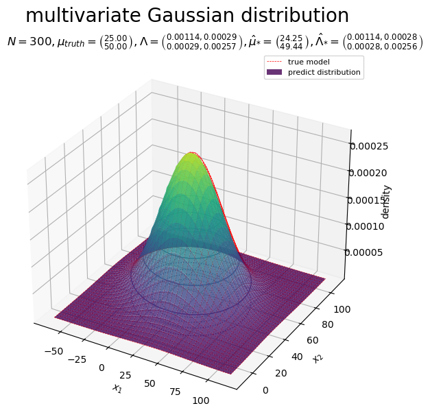
　真の分布(ガウス分布)を等高線や曲面(赤色・破線)、予測分布(ガウス分布)を等高線や曲面(グラデーション)で示す。

　データ数 $N$ が十分に大きいと、未観測データ $\mathbf{x}_{*}$ の予測分布 $\mathcal{N}(\mathbf{x}_{*} \mid \hat{\boldsymbol{\mu}}_{*}, \hat{\boldsymbol{\Lambda}}_{*}^{-1})$ の形状が真の分布 $\mathcal{N}(\mathbf{x}_{n,d} \mid \hat{\boldsymbol{\mu}}_{*}, \hat{\boldsymbol{\Lambda}}_{*}^{-1})$ に近付く。

　以上で、平均が未知の多次元ガウスモデルのベイズ推論を実装した。

学習の推移

　次は、平均が未知の多次元ガウス分布に対するベイズ推論を図で確認する。
　データ数を増やして分布の変化をアニメーションで確認する。
　作図コードについては「Suyama-Bayes/code/multivariate_gaussian_model/bayesian_inference/plot_parameter_updates_unknown_mean.py at master · anemptyarchive/Suyama-Bayes · GitHub」を参照のこと。

データ数と分布の関係

　データ数 $N$ を変化させたときの事後分布 $p(\boldsymbol{\mu} \mid \mathbf{X}, \boldsymbol{\Lambda}, \mathbf{m}, \boldsymbol{\Lambda}_{\mu})$ の変化をアニメーションにする。

　 $n$ 個のデータから求めた( $n$ 回更新した)事後分布(ガウス分布) $\mathcal{N}(\boldsymbol{\mu} \mid \mathbf{m}^{(n)}, \boldsymbol{\Lambda}_{\mu}^{(n)})$ を紫色の曲線(実線)、 $n$ 番目の観測データ $\mathbf{x}_n$ に対応する位置 $(\mu_1, \mu_2) = (x_{n,1}, x_{n,2})$ を桃色の点で示す。

　「ベイズ推論の実装」では、 $N$ 個(複数)のデータ $\mathbf{X}$ を用いて、事後分布のパラメータ $\hat{\mathbf{m}}, \hat{\boldsymbol{\Lambda}}_{\mu}$ を一括更新した。
　 $n$ 番目(1つ)のデータ $\mathbf{x}_n$ を用いて逐次更新する場合、 $n$ 回目の事後分布のパラメータ $\mathbf{m}^{(n)}, \boldsymbol{\Lambda}_{\mu}^{(n)}$ は、次の式で計算できる。

$\displaystyle \begin{aligned} \mathbf{m}^{(n)} &= (\boldsymbol{\Lambda}_{\mu}^{(n)})^{-1} \left( \boldsymbol{\Lambda}_{\mu}^{(n-1)} \mathbf{m}^{(n-1)} + \boldsymbol{\Lambda} \mathbf{x}_n \right) \\ \boldsymbol{\Lambda}_{\mu}^{(n)} &= \boldsymbol{\Lambda}_{\mu}^{(n-1)} + \boldsymbol{\Lambda} \end{aligned}$

　超パラメータの初期値(1回目の更新における事前分布のパラメータ)を $\mathbf{m}^{(0)}, \boldsymbol{\Lambda}_{\mu}^{(0)}$ として、 $\mathbf{m}^{(n-1)}, \boldsymbol{\Lambda}_{\mu}^{(n-1)}$ は、 $n-1$ 回目の更新における事後分布のパラメータであり、また $n$ 回目の更新における事前分布のパラメータを表す。

　データ数 $N$ が大きくなるのに応じて、パラメータ $\boldsymbol{\mu}$ の事後分布 $\mathcal{N}(\boldsymbol{\mu} \mid \hat{\mathbf{m}}, \hat{\boldsymbol{\Lambda}}_{\mu})$ のピークが真のパラメータ $\mu_{\mathrm{truth}}$ に近付いていくのを確認できる。

　データ数 $N$ を変化させたときの予測分布 $p(\mathbf{x}_{*} \mid \mathbf{X}, \boldsymbol{\Lambda}, \mathbf{m}, \boldsymbol{\Lambda}_{\mu})$ の変化をアニメーションにする。

　 $n$ 個のデータから求めた( $n$ 回更新した)予測分布(ガウス分布) $\mathcal{N}(\mathbf{x}_{*} \mid \hat{\boldsymbol{\mu}}_{*}, \hat{\boldsymbol{\Lambda}}_{*}^{-1})$ を紫色の曲線(実線)、 $n$ 番目の観測データ $\mathbf{x}_n$ を桃色の点で示す。

　「ベイズ推論の実装」では、 $N$ 個(複数)のデータ $\mathbf{X}$ を用いて、予測分布のパラメータ $\hat{\boldsymbol{\mu}}_{*}, \hat{\boldsymbol{\Lambda}}_{*}$ を一括更新した。
　 $n$ 番目(1つ)のデータ $\mathbf{x}_n$ を用いて逐次更新する場合、 $n$ 回目の予測分布のパラメータ $\boldsymbol{\mu}_{*}^{(n)}, \boldsymbol{\Lambda}_{*}^{(n)}$ は、次の式で計算できる。

$\displaystyle \begin{aligned} \boldsymbol{\mu}_{*}^{(n)} &= \mathbf{m}^{(n)} \\ \boldsymbol{\Lambda}_{*}^{(n)} &= \Bigl( (\boldsymbol{\Lambda}_{\mu}^{(n)})^{-1} + \boldsymbol{\Lambda}^{-1} \Bigr)^{-1} \end{aligned}$

　超パラメータの初期値 $\mathbf{m}^{(0)}, \boldsymbol{\Lambda}^{(0)}$ を用いて求めたパラメータを $\boldsymbol{\mu}_{*}^{(0)}, \boldsymbol{\Lambda}_{*}^{(0)}$ として、 $\boldsymbol{\mu}_{*}^{(n-1)}, \boldsymbol{\Lambda}_{*}^{(n-1)}$ は $n-1$ 回目の更新値を表す。

　データ数 $N$ が大きくなるのに応じて、未観測データ $\mathbf{x}_{*}$ の予測分布 $\mathcal{N}(\mathbf{x}_{*} \mid \hat{\boldsymbol{\mu}}_{*}, \hat{\boldsymbol{\Lambda}}_{*}^{-1})$ の形状が真の分布 $\mathcal{N}(\mathbf{x}_n \mid \boldsymbol{\mu}_{\mathrm{truth}}, \boldsymbol{\Lambda}^{-1})$ に近付いていくのを確認できる。

観測データと分布の関係

　データ数 $N$ の変化による観測データと事後分布、予測分布の関係をアニメーションにする。

　真の分布の期待値 $\mathbb{E}[\mathbf{x}_n]$ と真のパラメータ $\boldsymbol{\mu}_{\mathrm{truth}}$ の各図(分布)に対応する位置を赤色の直線(破線)、観測データの標本平均 $\bar{\mathbf{x}}$ を桃色の直線(破線)、事後分布の期待値 $\mathbb{E}[\boldsymbol{\mu}]$ と予測分布の期待値 $\mathbb{E}[\mathbf{x}_{*}]$ を紫色の直線(破線)で示す。

　生成分布(ガウス分布)、事後分布(ガウス分布)、予測分布(ガウス分布)の期待値は、それぞれ次の式で計算できる。

$\displaystyle \begin{aligned} \mathbb{E}_{\mathcal{N}(\mathbf{x}_n \mid \boldsymbol{\mu}_{\mathrm{truth}}, \boldsymbol{\Lambda}^{-1})}[\mathbf{x}_n] &= \boldsymbol{\mu}_{\mathrm{truth}} \\ \mathbb{E}_{\mathcal{N}(\boldsymbol{\mu} \mid \hat{\mathbf{m}}, \hat{\boldsymbol{\Lambda}}_{\mu}^{-1})}[\boldsymbol{\mu}] &= \hat{\mathbf{m}} \\ \mathbb{E}_{\mathcal{N}(\mathbf{x}_{*} \mid \hat{\boldsymbol{\mu}}_{*}, \hat{\boldsymbol{\Lambda}}_{*}^{-1})}[\mathbf{x}_{*}] &= \hat{\boldsymbol{\mu}}_{*} \\ &= \hat{\mathbf{m}} \end{aligned}$

　真の分布 $\mathcal{N}(\mathbf{x}_n \mid \boldsymbol{\mu}_{\mathrm{truth}}, \boldsymbol{\Lambda}^{-1})$ や真のパラメータ $\boldsymbol{\mu}_{\mathrm{truth}}$ と、観測データ $\mathbf{X}$ 、事後分布 $\mathcal{N}(\boldsymbol{\mu} \mid \hat{\mathbf{m}}, \hat{\boldsymbol{\Lambda}}_{\mu}^{-1})$ 、予測分布 $\mathcal{N}(\mathbf{x}_{*} \mid \hat{\boldsymbol{\mu}}_{*}, \hat{\boldsymbol{\Lambda}}_{*}^{-1})$ 、またそれぞれの統計量の対応関係を確認できる。

　以上で、平均が未知の多次元ガウスモデルのベイズ推論における学習推移を確認した。

　この記事では、平均が未知の場合の多次元ガウス分布に対するベイズ推論を扱った。次の記事では、精度が未知の場合を扱う。