This article is a comprehensive guide to state observers and state estimation in control systems. It covers the fundamental theory of Luenberger observers in both continuous-time and discrete-time settings, Kalman filters for stochastic estimation, robust H∞ filters using LMI-based design, and advanced topics including multi-rate state estimation and outlier-robust observers. Links to detailed articles, research papers, videos, and MATLAB codes are provided throughout.

Author: Hiroshi Okajima, Associate Professor, Kumamoto University, Japan — 20 years of control engineering research

MATLAB Codes: MATLAB_state_observer — Luenberger, Kalman, H∞, multi-rate, and outlier-robust observer codes (GitHub)

Why State Estimation Matters

In control systems, it is generally not possible to directly measure all internal states of a system. For example, a position sensor may be available, but velocity and acceleration must be estimated. A state observer (also called a state estimator or software sensor) is a mathematical algorithm that reconstructs the internal states of a dynamical system from its measured inputs and outputs.

State estimation plays a central role in modern control engineering:

State feedback control requires knowledge of all states, but sensors typically measure only a subset of outputs. Observers bridge this gap by estimating the unmeasured states.
Sensor fusion in robotics, autonomous vehicles, and IoT systems combines data from multiple sensors — often operating at different sampling rates — to produce a unified state estimate.
Fault detection and monitoring in industrial processes relies on comparing estimated states with expected behavior to identify anomalies. While dedicated fault detection algorithms are beyond the scope of this article, accurate state estimation is a prerequisite for such schemes.
Navigation and tracking systems such as GPS/INS integration use Kalman filters, a probabilistic form of state observer, as the core estimation engine.

This article serves as a hub connecting the various aspects of state estimation theory and practice. Each section below provides an overview with links to detailed articles for deeper study.

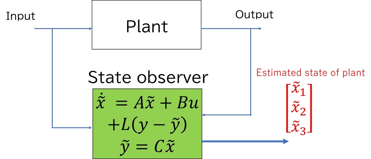
Continuous-Time State Observer (Luenberger Observer)

The most fundamental state observer is the Luenberger observer for continuous-time LTI systems. Consider a plant described by state equations:

$\displaystyle \dot{x}(t) = Ax(t) + Bu(t)$

$\displaystyle y(t) = Cx(t)$

where $x(t) \in \mathbb{R}^{n}$ is the state, $u(t) \in \mathbb{R}^{m}$ is the input, and $y(t) \in \mathbb{R}^{l}$ is the measured output. In many practical situations, only $y(t)$ is available, and the number of outputs $l$ is smaller than the state dimension $n$ .

The Luenberger observer constructs an estimate $\tilde{x}(t)$ of the state by running a copy of the plant model and correcting it using the output estimation error:

$\displaystyle \dot{\tilde{x}}(t) = A\tilde{x}(t) + Bu(t) + L\bigl(y(t) - C\tilde{x}(t)\bigr)$

Here, $L \in \mathbb{R}^{n \times l}$ is the observer gain matrix. The estimation error $e(t) = x(t) - \tilde{x}(t)$ satisfies:

$\displaystyle \dot{e}(t) = (A - LC)\,e(t)$

If the pair $(A, C)$ is observable, the gain $L$ can be designed so that $A - LC$ is stable with arbitrarily fast convergence. This is the dual of the state feedback pole placement problem: while state feedback places the poles of $A - BK$ , the observer places the poles of $A - LC$ .

Notation convention: Throughout this article, we write the observability pair as $(A, C)$ , following the convention in Kailath (1980) and many modern textbooks. Some authors write $(C, A)$ instead; the meaning is the same — it refers to the plant matrix $A$ and the output matrix $C$ whose observability is being assessed.

Observer-Based Feedback Control and the Separation Principle

A key theoretical result is the separation principle: when designing observer-based state feedback control for an LTI system, the state feedback gain $K$ and the observer gain $L$ can be designed independently. The closed-loop system using observer-based state feedback $u = -K\tilde{x}$ has $2n$ eigenvalues, consisting of the $n$ eigenvalues of $A - BK$ (determined by the controller design) and the $n$ eigenvalues of $A - LC$ (determined by the observer design). In practice, the observer poles are usually placed to converge faster than the controller poles, so that the state estimate converges quickly relative to the controlled response. A common guideline is to make the observer 2 to 5 times faster than the closed-loop controller dynamics.

For the detailed explanation and figures, see the blog article: State Observer for State Space Model

For the comprehensive treatment of state feedback design — including pole placement, LQR, integral-type servo systems, and the separation principle — see: State Feedback Control and State-Space Design: A Comprehensive Guide

MATLAB code: 01_luenberger_observer

Discrete-Time State Observer

Most practical control systems are implemented on digital computers, so the discrete-time formulation of observers is essential. Consider a discrete-time LTI system:

$\displaystyle x(k+1) = Ax(k) + Bu(k)$

$\displaystyle y(k) = Cx(k)$

The discrete-time Luenberger observer has the form:

$\displaystyle \tilde{x}(k+1) = A\tilde{x}(k) + Bu(k) + L\bigl(y(k) - C\tilde{x}(k)\bigr)$

The estimation error dynamics become:

$\displaystyle e(k+1) = (A - LC)\,e(k)$

For stability, all eigenvalues of $A - LC$ must lie inside the unit circle (not in the left-half plane as in the continuous-time case). Observer gain design can be performed via pole placement or LMI-based methods.

The discrete-time framework is particularly important because it directly connects to:

Kalman filter theory, which is formulated natively in discrete time
Multi-rate estimation problems, where different sensors sample at different discrete rates
Digital implementation of controllers and observers on microprocessors

For stability analysis and pole placement in discrete-time systems, see: Stability Analysis and Pole Placement Control for Discrete-Time Systems

For the relationship between continuous-time and discrete-time formulations, see: Discretization of Continuous-Time Control Systems

Observability: When Can We Estimate the State?

A fundamental prerequisite for state observer design is observability: the ability to uniquely determine the initial state from input-output measurements over a finite time interval.

For a discrete-time system with matrices $A$ and $C$ , observability is characterized by the observability matrix:

$\displaystyle \mathcal{O} = \begin{pmatrix} C \cr CA \cr CA^2 \cr \vdots \cr CA^{n-1} \end{pmatrix}$

The system is observable if and only if $\mathrm{rank}(\mathcal{O}) = n$ . A weaker condition, detectability, requires only that unobservable modes are stable. Detectability is sufficient for designing a stable observer.

For a detailed treatment including examples, see: Controllability and Observability of Systems

Observer Design: A Step-by-Step Numerical Example

To make the observer design process concrete, we walk through a simple numerical example of a discrete-time Luenberger observer for a second-order system.

Plant Model

Consider a discrete-time system with state dimension $n = 2$ , one input, and one output:

$\displaystyle A = \begin{pmatrix} 0 & 1 \cr -0.5 & 1.2 \end{pmatrix}, \quad B = \begin{pmatrix} 0 \cr 1 \end{pmatrix}, \quad C = \begin{pmatrix} 1 & 0 \end{pmatrix}$

This represents a system where only the first state $x_{1}(k)$ is measured, and the second state $x_{2}(k)$ must be estimated.

Step 1: Verify Observability

Compute the observability matrix:

$\displaystyle \mathcal{O} = \begin{pmatrix} C \cr CA \end{pmatrix} = \begin{pmatrix} 1 & 0 \cr 0 & 1 \end{pmatrix}$

Since $\mathrm{rank}(\mathcal{O}) = 2 = n$ , the system is observable, and the observer gain can place the error dynamics eigenvalues at any desired location.

Step 2: Choose Desired Observer Poles

The open-loop eigenvalues of $A$ are approximately $0.6 \pm 0.37j$ (inside the unit circle, so the plant is stable). A common design guideline is to make the observer 2 to 5 times faster than the plant dynamics. We choose the desired observer poles at:

$\displaystyle \mu_1 = 0.1, \quad \mu_2 = 0.2$

These are well inside the unit circle, ensuring fast convergence of the estimation error.

Step 3: Compute Observer Gain

The observer gain $L \in \mathbb{R}^{2 \times 1}$ must satisfy the characteristic equation:

$\displaystyle \det(zI - A + LC) = (z - \mu_1)(z - \mu_2) = z^2 - 0.3z + 0.02$

Let $L = \begin{pmatrix} l_{1} \cr l_{2} \end{pmatrix}$ . Then:

$\displaystyle A - LC = \begin{pmatrix} -l_1 & 1 \cr -0.5 - l_2 & 1.2 \end{pmatrix}$

Computing the characteristic polynomial of $zI - A + LC$ :

$\displaystyle \det(zI - A + LC) = \det \begin{pmatrix} z + l_1 & -1 \cr 0.5 + l_2 & z - 1.2 \end{pmatrix}$

$\displaystyle = (z + l_1)(z - 1.2) + (0.5 + l_2)$

$\displaystyle = z^2 + (l_1 - 1.2)z + (-1.2 l_1 + 0.5 + l_2)$

Matching coefficients with $z^{2} - 0.3z + 0.02$ :

$\displaystyle l_1 - 1.2 = -0.3 \implies l_1 = 0.9$

$\displaystyle -1.2(0.9) + 0.5 + l_2 = 0.02 \implies l_2 = 0.6$

The observer gain is:

$\displaystyle L = \begin{pmatrix} 0.9 \cr 0.6 \end{pmatrix}$

Step 4: Observer Implementation

The observer equation is:

$\displaystyle \tilde{x}(k+1) = A\tilde{x}(k) + Bu(k) + L\bigl(y(k) - C\tilde{x}(k)\bigr)$

which expands to:

$\displaystyle \tilde{x}(k+1) = (A - LC)\tilde{x}(k) + Bu(k) + Ly(k)$

$\displaystyle = \begin{pmatrix} -0.9 & 1 \cr -1.1 & 1.2 \end{pmatrix} \tilde{x}(k) + \begin{pmatrix} 0 \cr 1 \end{pmatrix} u(k) + \begin{pmatrix} 0.9 \cr 0.6 \end{pmatrix} y(k)$

For more examples including simulation results and MATLAB implementation, see: State Observer: Understanding the Basic Mechanism and State Observer for State Space Model

MATLAB code: 01_luenberger_observer — includes this example with simulation and plotting code

Kalman Filter: Optimal Stochastic State Estimation

The Kalman filter extends the deterministic observer framework to stochastic systems by incorporating statistical models of process noise and measurement noise. Consider the discrete-time stochastic system:

$\displaystyle x(k+1) = Ax(k) + Bu(k) + B_d w(k)$

$\displaystyle y(k) = Cx(k) + v(k)$

where $w(k)$ is process noise with covariance $Q$ and $v(k)$ is measurement noise with covariance $R$ , both assumed to be zero-mean white Gaussian noise sequences. The matrix $B_{d}$ maps the process noise into the state equation; it may differ from the input matrix $B$ because the noise may enter through different channels than the control input. This noise model will be extended in the H∞ filter section below, where a unified disturbance input is used instead of separate process and measurement noise terms.

The Kalman filter provides the minimum mean-squared error estimate of the state. It operates in two steps at each time instant:

Prediction step — propagate the state estimate and error covariance forward in time using the system model:

$\displaystyle \hat{x}(k|k-1) = A\hat{x}(k-1|k-1) + Bu(k-1)$

$\displaystyle P(k|k-1) = AP(k-1|k-1)A^T + B_d Q B_d^T$

Update step — incorporate the new measurement to correct the prediction:

$\displaystyle K_f(k) = P(k|k-1)C^T \bigl(CP(k|k-1)C^T + R\bigr)^{-1}$

$\displaystyle \hat{x}(k|k) = \hat{x}(k|k-1) + K_f(k)\bigl(y(k) - C\hat{x}(k|k-1)\bigr)$

$\displaystyle P(k|k) = \bigl(I - K_f(k)C\bigr)P(k|k-1)$

Here, $P(k|k)$ is the error covariance matrix, and $K_{f}(k)$ is the Kalman gain that optimally balances the model prediction against the noisy measurement. When the noise covariances $Q$ and $R$ are known and the system satisfies the conditions that $(A, B_{d})$ is stabilizable and $(A, C)$ is detectable, the Kalman gain converges to a steady-state value, yielding a time-invariant observer structure similar to the Luenberger observer. The stabilizability of $(A, B_{d})$ ensures that the Riccati equation has a stabilizing solution, while the detectability of $(A, C)$ ensures that the resulting observer is stable.

The Kalman filter is widely used in navigation (GPS/INS), robotics, economics, and signal processing. It is also the basis for extensions such as the Extended Kalman Filter (EKF) for nonlinear systems and the Unscented Kalman Filter (UKF) for improved accuracy in strongly nonlinear settings.

For the detailed article on Kalman filters, see: Kalman Filter: From Basic Algorithm to Multi-Rate Extensions

MATLAB code: 03_kalman_filter

H-infinity Filter: Robust State Estimation Using LMI

When precise statistical models of noise are unavailable, the H∞ filter (also called the minimax or worst-case optimal filter) provides an alternative to the Kalman filter. Instead of minimizing the mean-squared error under Gaussian noise assumptions, the H∞ filter minimizes the worst-case ratio of estimation error energy to disturbance energy.

The system model for H∞ filter design uses a unified disturbance formulation. The process noise and measurement noise from the Kalman filter section are combined into a single disturbance input $w(k)$ :

$\displaystyle x(k+1) = Ax(k) + Bu(k) + B_d w(k)$

$\displaystyle y(k) = Cx(k) + Dw(k)$

Here, the matrix $D$ maps the disturbance directly to the measurement output, playing a role analogous to the measurement noise $v(k)$ in the Kalman filter formulation. The key difference from the Kalman filter model is that $w(k)$ is not assumed to be Gaussian — it is only assumed to have bounded energy.

The H∞ filter design seeks an observer gain $L$ such that the transfer function from $w$ to the estimation error $e = x - \tilde{x}$ satisfies:

$\displaystyle \|T_{w \to e}\|_\infty \lt \gamma$

for a specified performance level $\gamma \gt 0$ . This can be formulated as a Linear Matrix Inequality (LMI) feasibility problem, which can be solved efficiently using standard convex optimization tools such as MATLAB's LMI Toolbox or YALMIP.

The LMI-based design approach offers several advantages:

No Gaussian assumption: the H∞ filter guarantees performance for any bounded-energy disturbance, not just Gaussian noise.
Flexible design objectives: additional constraints (e.g., pole placement, structural constraints) can be incorporated as additional LMIs.
Direct extension to time-varying and multirate systems: the LMI framework naturally accommodates periodic Lyapunov functions needed for multirate observer design.

For the fundamentals of LMI-based controller and observer design, see: Design of Controller Parameters Using Linear Matrix Inequalities in MATLAB

For advanced LMI techniques including Schur's lemma and variable elimination, see: Advanced LMI Techniques in Control System Design

For the detailed article, see: H∞ Filter: Robust State Estimation Using LMI Optimization

MATLAB code: 04_hinf_filter

Multi-Rate State Estimation

In many practical systems, multiple sensors operate at different sampling rates. For example, in mobile robot control, a camera may produce images at 30 Hz, an IMU at 200 Hz, and a GPS receiver at 1 Hz. Designing a state observer that correctly handles these heterogeneous sampling rates is a non-trivial problem.

The multi-rate observer framework models the observation structure using a periodically time-varying diagonal matrix $V_{k}$ that indicates which sensors are active at each time step:

$\displaystyle y(k) = V_k C x(k) + V_k D u(k)$

$\displaystyle V_{k} = \mathrm{diag}[v_{1}(k), \ldots, v_{l}(k)$ ]

where $v_{i}(k) = 1$ when sensor $i$ is observed and $v_{i}(k) = 0$ otherwise. The frame period $M$ is the least common multiple of all individual sensor periods $M_{1}, \ldots, M_{l}$ .

The observer takes the form of a periodically time-varying system:

$\displaystyle \tilde{x}(k+1) = A\tilde{x}(k) + Bu(k) + L_k\bigl(y(k) - V_k C\tilde{x}(k)\bigr)$

where the observer gain $L_{k}$ varies periodically with period $M$ , adapting to the time-varying observation structure. The gain design can be performed using cyclic reformulation, which transforms the periodically time-varying system into an equivalent LTI system of higher dimension. With this reformulation, standard LMI-based techniques can be applied to design the observer gain while optimizing performance criteria such as the $\ell_{2}$ -induced norm of the estimation error.

Key results from the multi-rate observer design include:

The observer is a periodically time-varying system with period $M$ , naturally matching the multi-rate sensor structure.
LMI conditions involving periodic Lyapunov matrices ensure stability and performance of the estimation error dynamics.
The framework accommodates systems where observability varies across sampling instants — at some time steps, insufficient sensor data is available to reconstruct all states, but the observer accumulates information over the full period.

For the detailed design method using LMI optimization, see: State Observer Under Multi-Rate Sensing Environment and Its Design Using l2-Induced Norm

For the system identification method that provides the plant model needed for multi-rate observer design, see: System Identification Under Multirate Sensing Environments (see also the JRM 2025 paper)

MATLAB code: 05_multirate_observer, 06_multirate_feedback, 07_multirate_kalman

Outlier-Robust State Estimation: MCV Observer

Standard observers and Kalman filters assume that sensor measurements are corrupted by noise with bounded variance. However, in practice, sensor outputs may contain outliers — sudden, large-magnitude errors caused by sensor malfunctions, environmental disturbances, or communication failures. Even a single outlier can drastically degrade the estimation accuracy of conventional observers.

The MCV (Median of Candidate Vectors) observer addresses this problem by constructing multiple candidate state estimates from different time instants and selecting the best estimate using a median operation. More precisely, at each time step $k$ , the MCV observer:

Generates $F_{1}$ candidate state estimates, each computed from the output at a different past time instant using a deadbeat-type computation:

$\displaystyle \hat{x}_i(k) = A^{F_1 - i}\tilde{x}(k - F_1) + G_i u_{k-i:k} + H_i y(k-i)$

where $G_{i}$ and $H_{i}$ are matrices depending on the system parameters.

Applies the element-wise median operation to these candidates:

$\displaystyle \tilde{x}_{\mathrm{med}}(k) = \mathrm{med}\bigl(\hat{x}_1(k), \hat{x}_2(k), \ldots, \hat{x}_{F_1}(k)\bigr)$

which naturally rejects outlier-contaminated estimates.

Feeds the median estimate into a stabilizing observer to obtain the final estimate. The observer gain can be designed using LMI optimization to guarantee estimation performance.

The MCV observer is robust to outliers as long as the number of outliers within any window of $F_{1}$ time steps does not exceed $F_{2}$ , where $F_{2} \lt F_{1}/2$ . This condition ensures that the median operation always selects from non-corrupted candidates.

For the concept and algorithm of the MCV observer, see: State Estimator Unaffected by Sensor Outliers: MCV Approach

For the detailed paper explanation and numerical examples, see: State Estimation Method Using Median of Multiple Candidates for Observation Signals Including Outliers

MATLAB code: 08_mcv_observer

Comparison of Observer Design Methods

The following table summarizes the key characteristics of the state estimation methods discussed in this article.

Method	Noise Model	Optimality	Design Tool	Key Advantage
Luenberger Observer	Deterministic (no noise model)	Pole placement	Eigenvalue assignment	Simplicity, intuitive design
Kalman Filter	Gaussian (known Q, R)	Minimum variance	Riccati equation	Optimal for Gaussian noise
H∞ Filter	Bounded energy (unknown distribution)	Worst-case optimal	LMI	Robust to model uncertainty
Multi-Rate Observer	Periodic time-varying	LMI-based	Periodic LMI	Handles heterogeneous sensor rates
MCV Observer	Outlier-contaminated	Median-based robustness	LMI	Tolerates large sporadic outliers

How to Choose the Right Observer

With several observer design methods available, choosing the right one for a given application is a practical decision that depends on the noise environment, available computational resources, and performance requirements. The following guide summarizes the key considerations.

Start from your noise model. If precise statistical information about the process and measurement noise is available (i.e., the covariance matrices $Q$ and $R$ are known), the Kalman filter is the natural first choice because it provides the minimum-variance estimate. If only bounds on the noise energy are known but its statistical distribution is uncertain, the H∞ filter provides guaranteed worst-case performance without relying on Gaussian assumptions. If the measurements may contain occasional large outliers (e.g., sensor glitches or communication dropouts), the MCV observer is specifically designed to reject such anomalies.

Consider the sensor configuration. If all sensors operate at the same sampling rate, any of the above methods can be applied directly. If sensors have different sampling rates (e.g., camera at 30 Hz, IMU at 200 Hz, GPS at 1 Hz), the multi-rate observer framework is required to correctly handle the heterogeneous observation structure.

Evaluate the design complexity. The Luenberger observer is the simplest to implement and understand, requiring only pole placement. It serves as an excellent starting point for prototyping and education, but does not explicitly account for noise. The Kalman filter adds optimality at the cost of requiring noise covariance tuning. The H∞ filter and multi-rate observer involve LMI-based optimization, which offers more flexibility but requires familiarity with LMI tools.

The decision can be summarized as follows:

Question	Yes → Method	No → Next Question
Are noise covariances $Q, R$ reliably known?	Kalman Filter	↓
Is worst-case robustness more important than average-case optimality?	H∞ Filter	↓
Do sensors operate at different sampling rates?	Multi-Rate Observer	↓
Are sensor outliers a concern?	MCV Observer	↓
Is simplicity the priority?	Luenberger Observer	—

In practice, these methods are often combined. For example, a multi-rate Kalman filter handles both stochastic noise and heterogeneous sensor rates, and an identified model (obtained via system identification) can be refined using a Model Error Compensator (MEC) to improve robustness against model uncertainty.

State estimation connects to many other areas in control engineering:

State feedback control and state-space design — The observer provides the estimated state needed for state feedback. The separation principle guarantees that the controller and observer can be designed independently. For the comprehensive treatment of pole placement, LQR, integral-type servo systems, and the separation principle, see: State Feedback Control and State-Space Design: A Comprehensive Guide. For individual topics, see also: State Feedback Control: Design Gains using Pole Placement and State Feedback Control: Design Gains using Optimal Regulators
Model Error Compensator (MEC) — When there is a gap between the plant model used in observer design and the actual plant, the MEC framework can improve robustness by compensating for model errors. The MEC can be combined with observer-based control to enhance performance. See: Model Error Compensator (MEC)
System identification — Before designing an observer, a mathematical model of the plant is required. System identification techniques provide this model from measured input-output data. See: System Identification: From Data to Dynamical Models
State-space model — The mathematical framework for all observer designs discussed in this article. See: State-Space Model for Control

Frequently Asked Questions

Q: What is the difference between a state observer and a state estimator?

The terms are often used interchangeably. In the control engineering literature, "state observer" typically refers to the deterministic framework (Luenberger observer), while "state estimator" may emphasize the stochastic setting (Kalman filter). Both reconstruct the internal states of a system from measured inputs and outputs. In practice, the distinction is largely historical.

Q: When should I use a Kalman filter instead of a Luenberger observer?

Use a Kalman filter when you have a reasonable statistical model of the process noise and measurement noise (i.e., their covariance matrices $Q$ and $R$ ). The Kalman filter optimally balances the model prediction and the noisy measurement. If noise statistics are unknown or hard to estimate, consider the H∞ filter, which does not require Gaussian assumptions. See the Kalman Filter article and the H∞ Filter article for detailed comparisons.

Q: What does "observable" mean, and why is it important?

A system is observable if its entire internal state can be uniquely determined from a finite sequence of input and output measurements. Mathematically, this requires the observability matrix to have full rank. If a system is not observable, some internal states cannot be reconstructed by any observer, regardless of the gain design. A weaker condition called detectability (unobservable modes are stable) is sufficient for designing a stable observer. See: Controllability and Observability of Systems

Q: How do I choose observer pole locations?

A common guideline is to place the observer poles 2 to 5 times faster than the closed-loop controller poles. In discrete time, this means the observer eigenvalues should have smaller magnitude (closer to the origin) than the plant eigenvalues. However, excessively fast poles amplify measurement noise, so there is a trade-off between convergence speed and noise sensitivity. LMI-based design methods can systematically optimize this trade-off. See: LMIs and Controller Design

Q: Can I design an observer if my sensors have different sampling rates?

Yes. The multi-rate observer framework handles sensors with heterogeneous sampling rates by modeling the observation structure using periodically time-varying matrices. The observer gain is designed using cyclic reformulation and LMI optimization. This approach is described in detail in the Multi-Rate Observer article.

Q: What if my sensor occasionally produces completely wrong values (outliers)?

Standard observers and Kalman filters are sensitive to outliers because they trust every measurement. The MCV (Median of Candidate Vectors) observer addresses this by generating multiple candidate estimates and selecting the best one via a median operation, which naturally rejects outlier-contaminated measurements. See: MCV Observer

Q: Do I need a plant model before designing an observer?

Yes. All observer design methods require a mathematical model of the plant (the matrices $A, B, C, D$ in state-space form). This model can be obtained through first-principles modeling or through system identification from measured data. See: System Identification: From Data to Dynamical Models

Q: Can the observer and controller be designed independently?

Yes, under the separation principle. For linear systems, the state feedback gain and the observer gain can be designed independently, and the resulting closed-loop eigenvalues are the union of the controller poles and the observer poles. This principle simplifies the design process significantly. See: State Observer for State Space Model

Summary

This article has provided an overview of the major state estimation methods in control engineering. The Luenberger observer forms the deterministic foundation, the Kalman filter extends this to optimal stochastic estimation, and the H∞ filter provides robustness when noise statistics are uncertain. For systems with heterogeneous sensor rates, the multi-rate observer framework offers a principled solution using cyclic reformulation and periodic LMI design. When sensor outliers are a concern, the MCV observer provides robustness through median-based candidate selection. The comparison table and selection guide in this article can help practitioners choose the appropriate method for their application.

Each method is supported by detailed spoke articles, MATLAB codes, and research papers linked throughout. As future work, extensions to nonlinear state estimation (EKF, UKF, Particle Filter) and disturbance estimation (Unknown Input Observer, Disturbance Observer) will be added to this hub article.

Key References

The following are foundational references in state estimation and observer theory.

Observer Theory:

D.G. Luenberger, Observing the State of a Linear System, IEEE Transactions on Military Electronics, Vol. 8, No. 2, pp. 74–80, 1964.

D.G. Luenberger, An Introduction to Observers, IEEE Transactions on Automatic Control, Vol. 16, No. 6, pp. 596–602, 1971.

Kalman Filter and Optimal Filtering:

R.E. Kalman, A New Approach to Linear Filtering and Prediction Problems, Trans. ASME J. Basic Engineering, Vol. 82, No. 1, pp. 35–45, 1960.

B.D.O. Anderson and J.B. Moore, Optimal Filtering, Prentice-Hall, 1979.

LMI-Based Design:

S. Boyd, L. El Ghaoui, E. Feron, and V. Balakrishnan, Linear Matrix Inequalities in System and Control Theory, SIAM, 1994.

Periodic Systems and Cyclic Reformulation:

S. Bittanti and P. Colaneri, Invariant Representations of Discrete-Time Periodic Systems00087-X), Automatica, Vol. 36, No. 12, pp. 1777–1793, 2000.

S. Bittanti, P. Colaneri, and G. De Nicolao, The Difference Periodic Riccati Equation for the Periodic Prediction Problem, IEEE Trans. Automatic Control, Vol. 33, No. 8, pp. 706–712, 1988.

Author's Papers on Advanced State Estimation:

H. Okajima, Y. Hosoe, and T. Hagiwara, State Observer Under Multi-Rate Sensing Environment and Its Design Using l2-Induced Norm, IEEE Access, Vol. 11, pp. 21190–21200, 2023.

H. Okajima, K. Arinaga, and A. Hayashida, Design of observer-based feedback controller for multi-rate systems with various sampling periods using cyclic reformulation, IEEE Access, Vol. 11, pp. 127573–127583, 2023.

H. Okajima, State Estimation Method Using Median of Multiple Candidates for Observation Signals Including Outliers, SICE Journal of Control, Measurement, and System Integration (JCMSI), Vol. 14, No. 2, pp. 245–254, 2021.

Modern Textbooks:

D. Simon, Optimal State Estimation: Kalman, H∞, and Nonlinear Approaches, Wiley, 2006.

Blog Articles (blog.control-theory.com)

Fundamentals: - State Observer for State Space Model — Basic concept of Luenberger observer - Controllability and Observability of Systems — Prerequisites for observer design - State-Space Model for Control — State equation representation - Stability Analysis and Pole Placement Control for Discrete-Time Systems - Discretization of Continuous-Time Control Systems

Design Tools: - Design of Controller Parameters Using Linear Matrix Inequalities in MATLAB - Advanced LMI Techniques in Control System Design

Research: - State Observer Under Multi-Rate Sensing Environment (IEEE ACCESS 2023) - State Estimation Method Using Median of Multiple Candidates for Observation Signals Including Outliers (SICE JCMSI 2021) - State Estimator Unaffected by Sensor Outliers: MCV Approach

Research Web Pages (www.control-theory.com)

Multi-rate System / MCV Observer for Overcoming Outliers / Linear Matrix Inequality / Model Error Compensator / Publications

Video

State Observer Basics (English):

Research on Advanced State Estimation (English):

Japanese Video Portal (日本語):

YouTube: Control Engineering Channel / Video Portal / State Estimation Videos

Video Portal

制御工学チャンネル — 動画ポータルサイト: 状態推定（in Japanese）

MATLAB Code (GitHub)

All MATLAB codes for the methods discussed in this article are available in a single repository:

MATLAB_state_observer — Luenberger observer, Kalman filter, H∞ filter, multi-rate observer/feedback/Kalman, and MCV observer.

Additional external code links: - MATLAB File Exchange: State Estimation under Multi-Rate Sensing: IEEE ACCESS 2023 / Outlier-Robust State Estimator: JCMSI 2021 - Code Ocean: Multi-Rate System Code

Self-Introduction

Hiroshi Okajima — Associate Professor, Graduate School of Science and Technology, Kumamoto University. Member of SICE, ISCIE, and IEEE.

www.control-theory.com / Blog / YouTube / GitHub

If you found this article helpful, please consider bookmarking or sharing it.

StateObserver #StateEstimation #KalmanFilter #LuenbergerObserver #HinfinityFilter #LMI #MultiRateSystems #RobustEstimation #ControlEngineering #SensorFusion