This article explains how to add robustness to PID control systems using the Model Error Compensator (MEC). PID control is the most widely used controller in industrial applications, but its performance degrades when the plant model contains errors or when disturbances act on the system. MEC provides a simple add-on structure that makes existing PID control systems robust against model uncertainty — without modifying the PID controller itself. Related articles, related papers, and MATLAB links are placed at the bottom.
Author: Hiroshi Okajima, Associate Professor, Kumamoto University, Japan — 20 years of control engineering research
This article is based on the following comprehensive paper.
- Okajima, Model Error Compensator for adding Robustness toward Existing Control Systems, IFAC PapersOnLine, Vol. 56, Issue 2, pp. 3998–4005 (2023) (Free access, Elsevier)
- Why Add Robustness to PID Control?
- MEC + PID: System Structure
- Effective Plant with MEC
- Error Compensator Design for PID + MEC
- Numerical Simulation: PID + MEC
- MATLAB Code
- When to Use PID + MEC
- Connections to Related Research
- MATLAB Code
- Related Articles and Videos
- Paper Information
- ModelErrorCompensator #MEC #PIDControl #RobustControl #ControlEngineering #Robustness #MATLAB #AddOnCompensator #ParameterVariation #IndustrialControl
Why Add Robustness to PID Control?
PID (Proportional-Integral-Derivative) control is the dominant controller in industrial process control, mechatronics, and robotics. Its simplicity and intuitive tuning make it attractive, but PID controllers are inherently designed for a specific nominal model. When the actual plant differs from this model due to parameter variations, aging, load changes, or unmodeled dynamics, PID performance can degrade significantly.
Common approaches to address this problem include:
- Re-tuning PID gains — requires access to the plant and re-identification, which may not always be feasible
- Robust PID design — designs PID gains that account for uncertainty from the start, but often sacrifices nominal performance for robustness
- Switching to advanced controllers — replaces PID entirely with H-infinity, MPC, or adaptive control, losing the simplicity of PID
The Model Error Compensator offers a fundamentally different approach: keep the existing PID controller unchanged and add a compensator that makes the plant behave like the nominal model. This "add-on" philosophy is especially practical because:
- The existing PID controller, which was carefully tuned for the nominal plant, remains untouched
- The MEC can be designed independently of the PID controller
- If the MEC is removed, the system reverts to the original PID control system
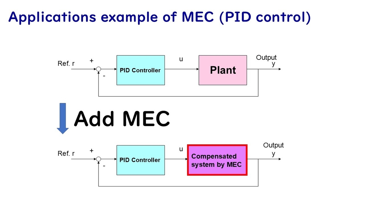
MEC + PID: System Structure
Standard PID Control (Without MEC)
In a standard PID control system, the controller is applied directly to the actual plant
:
The closed-loop system with unit feedback gives:
where is the reference input and
is the output. When the actual plant
differs from the nominal model
, the closed-loop performance deviates from the designed behavior.
Adding MEC to PID Control
The MEC is placed between the PID controller output and the actual plant input. The structure consists of:
- Nominal model
— the plant model used when designing the PID controller
- Error compensator
— a feedback compensator that drives the plant output toward the model output
The compensated control input is:
where is the PID controller output. The error signal
represents the difference between the actual plant output and the model output. The error compensator
feeds this difference back to correct the control input.
The key point: The PID controller sees the compensated plant (plant + MEC) rather than the raw plant. When MEC works effectively, the compensated plant behaves like
, so the PID controller operates as if the plant were the nominal model.
Block Diagram
The overall structure of MEC + PID is:
r(s) → [PID: C(s)] → u(s) → [MEC] → u_c(s) → [Plant: P(s)] → y(s)
                                ↑                                  |
                                |    [Model: P_n(s)] ←─── u_c(s)  |
                                |         |                        |
                                |    y_m(s)                        |
                                |         |                        |
                                └── D(s) ← (y - y_m) ─────────────┘
The image below from the hub article illustrates this integration.
Effective Plant with MEC
The transfer function from to
through the MEC-compensated plant is:
This is the effective plant that the PID controller sees. When the error compensator gain is sufficiently large (high-gain feedback), the effective plant approaches the nominal model:
In practice, making infinitely large is not possible due to sensor noise amplification. The design of
involves a trade-off between robustness (large gain) and noise sensitivity (limited gain).
Error Compensator Design for PID + MEC
Basic Design: PI-Type Error Compensator
For the simplest case of a SISO minimum-phase plant with relative degree 1, the error compensator can be designed as a PI controller:
where and
are the proportional and integral gains of the error compensator. The integral term ensures zero steady-state model error. The gains should be set sufficiently large to achieve effective error compensation, while keeping noise amplification within acceptable limits.
Design Considerations
When designing the error compensator for a PID + MEC system:
- Minimum phase systems: High-gain PI or PID-type error compensators work well. Increasing the gains improves robustness.
- Non-minimum phase systems: High-gain feedback may destabilize the error compensation loop. In this case, a parallel feedforward compensator can be added to convert the effective system to minimum phase. See the related article on MEC for Non-Minimum Phase Systems.
- Sensor noise: The error compensator amplifies sensor noise. For systems with significant noise, the gain must be limited, and LMI-based design methods can optimize the trade-off between robustness and noise rejection.
For detailed design methodologies including LMI-based approaches and particle swarm optimization, see the MEC hub article.
Numerical Simulation: PID + MEC
Problem Setup
Consider a control plant with parameter variations:
where , and
. This is an unstable plant (pole at
).
The PID controller (proportional only in this example) is , which stabilizes the nominal plant
.
The error compensator is designed as:
This is a PI-type error compensator with high gains (,
).
Results: Without MEC
When 10 random parameter variations are applied without MEC, the step responses show significant variation:
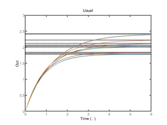
The response varies significantly depending on the parameter values, demonstrating the sensitivity of the PID controller to model uncertainty.
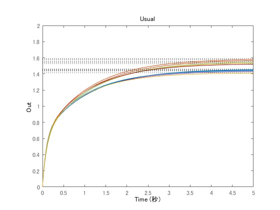
Results: With MEC
With the MEC added, the same 10 parameter variations produce nearly identical responses:

The MEC successfully suppresses the effect of parameter variations, making the closed-loop system behave consistently regardless of the actual plant parameters.
Second Example: 2nd-Order Unstable System
A more complex control plant is also considered:
with and
. The proportional controller is
.

Again, the MEC effectively suppresses the effect of parameter variations on the closed-loop response.
MATLAB Code
The following MATLAB code demonstrates the PID + MEC simulation for the first example (unstable plant).
clear;
close all;
a = 1;
b = 1;
for i = 1:10
    delb = -0.1+0.2*rand();
    dela = -0.1+0.2*rand();
    P = tf([b+delb],[1 -a-dela]);
    Pn = tf([b],[1 -a]);
    C = 2;
    D = tf([50 50],[1 0]);
    % Without MEC
    figure(1)
    step(feedback(P*C,1))
    hold on
    % With MEC
    figure(2)
    step(feedback(Pn*C,1)*feedback(P*D,1) - feedback(C,Pn)*feedback(P,D))
    hold on
end
Additional MATLAB code for PID + MEC integration is available at:
- GitHub: Hiroshi-Okajima/MEC05-rengo2022
When to Use PID + MEC
PID + MEC is particularly effective in the following scenarios:
- Existing PID systems that cannot be re-tuned: When a PID controller is already deployed and working in nominal conditions, MEC can be added without changing the PID gains.
- Plants with parameter variations: When plant parameters change over time (e.g., temperature-dependent dynamics, wear), MEC continuously compensates for these changes.
- Plants with uncertain dynamics: When the plant model is approximate and the true dynamics are not precisely known.
- Rapid prototyping: When a quick robustness improvement is needed without extensive re-design of the control system.
The MEC approach can be viewed as a form of two-degree-of-freedom (2-DOF) control, where the PID controller handles tracking performance and the MEC handles robustness. However, unlike conventional 2-DOF design where both parts are designed simultaneously, MEC allows the PID and the error compensator to be designed independently.
Connections to Related Research
Model Error Compensator: Comprehensive Guide — For the full overview of MEC including its basic structure, design philosophy, and various extensions, see the MEC hub article.
MEC vs Disturbance Observer — For a structural comparison between MEC and the Disturbance Observer (DOB), including when to use which, see Model Error Compensator vs Disturbance Observer: A Structural Comparison. The DOB also achieves robustness for PID control, but requires an inverse model that may not exist for non-minimum phase systems.
MEC for Non-Minimum Phase Systems — When the plant has unstable zeros, high-gain error compensation is not directly applicable. A parallel feedforward compensator approach resolves this issue. See MEC for Non-Minimum Phase Systems.
MEC for Nonlinear Systems — MEC enables robust feedback linearization for nonlinear systems, providing an output-feedback type linearization method. See MEC for Nonlinear Systems: Robust Feedback Linearization.
MEC Design with LMI — For systems with polytopic uncertainty, LMI-based design of the error compensator provides systematic robustness guarantees. The MATLAB code is available at GitHub: Robust-control-MATLAB_MEC01.
IFAC 2023 Paper — H. Okajima, Model Error Compensator for adding Robustness toward Existing Control Systems, IFAC PapersOnLine, Vol. 56, Issue 2, pp. 3998–4005 (2023). This paper provides a comprehensive overview of MEC including the PID integration example.
MATLAB Code
- GitHub (PID + MEC): MEC05-rengo2022
- GitHub (Basic MEC with LMI): Robust-control-MATLAB_MEC01
- GitHub (Sensor Noise Trade-off): MATLAB_MEC02_sensor_noise
Related Articles and Videos
Blog Articles (blog.control-theory.com)
- Model Error Compensator (MEC): Enhance the Robustness of Existing Control Systems
- Model Error Compensator vs Disturbance Observer: A Structural Comparison
- System Identification: Obtaining Dynamical Model
- Linear Matrix Inequalities (LMIs) and Controller Design
- Discretization of Continuous-Time Control Systems
Research Web Pages (www.control-theory.com)
Video
Paper Information
- Okajima, "Model Error Compensator for adding Robustness toward Existing Control Systems", IFAC PapersOnLine, Vol. 56, Issue 2, pp. 3998–4005, 2023. DOI: 10.1016/j.ifacol.2023.10.1098 (Free access)
Self-Introduction
Hiroshi Okajima — Associate Professor, Graduate School of Science and Technology, Kumamoto University. Member of SICE, ISCIE, and IEEE.
If you found this article helpful, please consider bookmarking or sharing it.