This article provides a comprehensive explanation of the $H_\infty$ filter (H-infinity filter) for robust state estimation in control systems. Unlike the Kalman filter, the $H_\infty$ filter does not require knowledge of noise statistics and instead minimizes the worst-case estimation error. The article covers the problem formulation, LMI-based design, comparison with the Kalman filter, and extensions to discrete-time and multi-rate systems. Related articles, research papers, and MATLAB links are placed at the bottom.

Author: Hiroshi Okajima, Associate Professor, Kumamoto University, Japan — 20 years of control engineering research

For the overview of state estimation methods, see the hub article: State Observer and State Estimation: A Comprehensive Guide

For the Kalman filter approach, see: Kalman Filter: From Basic Algorithm to Multi-Rate Extensions

Why the H-infinity Filter?

The Kalman filter is the optimal state estimator when the process noise and measurement noise are Gaussian with known covariance matrices $Q$ and $R$ . However, in many practical situations:

The noise statistics are unknown or poorly characterized
The noise may be non-Gaussian (e.g., bounded-energy disturbances, structured uncertainty)
The plant model contains parametric uncertainty
Worst-case performance guarantees are more important than average-case optimality

In such situations, the $H_\infty$ filter provides a robust alternative. Instead of minimizing the mean-squared estimation error (as the Kalman filter does), the $H_\infty$ filter minimizes the worst-case ratio of the estimation error energy to the disturbance energy, over all possible disturbance signals with finite energy. This makes the $H_\infty$ filter inherently robust to model uncertainty and unknown noise characteristics.

Problem Formulation

System Model

Consider the discrete-time LTI system:

$\displaystyle x(k+1) = Ax(k) + Bu(k) + B_d w(k)$

$\displaystyle y(k) = Cx(k) + Dw(k)$

$\displaystyle z(k) = C_z x(k)$

where:

$x(k) \in \mathbb{R}^{n}$ is the state vector
$u(k) \in \mathbb{R}^{m}$ is the known control input
$y(k) \in \mathbb{R}^{l}$ is the measured output
$w(k) \in \mathbb{R}^{p}$ is the generalized disturbance (encompassing process noise, measurement noise, and any other unknown signals)
$z(k) \in \mathbb{R}^{r}$ is the estimation target (the signal we want to estimate)
$A, B, B_{d}, C, D, C_{z}$ are system matrices of appropriate dimensions

The generalized disturbance $w(k)$ is assumed only to have finite energy:

$\displaystyle \sum_{k=0}^{\infty} w(k)^T w(k) < \infty$

No statistical assumptions are made — $w(k)$ can be any signal in $\ell_{2}$ .

Observer Structure

The observer has the standard Luenberger form:

$\displaystyle \hat{x}(k+1) = A\hat{x}(k) + Bu(k) + L\bigl(y(k) - C\hat{x}(k)\bigr)$

where $L \in \mathbb{R}^{n \times l}$ is the observer gain to be designed. The estimation error is $e(k) = x(k) - \hat{x}(k)$ , and the estimation output error is $\tilde{z}(k) = z(k) - C_{z}\hat{x}(k) = C_{z} e(k)$ .

H-infinity Performance Criterion

The $H_\infty$ filter design seeks an observer gain $L$ such that the worst-case gain from the disturbance $w$ to the estimation error $\tilde{z}$ is bounded by a prescribed level $\gamma > 0$ :

$\displaystyle \|T_{w \to \tilde{z}}\|_\infty := \sup_{w \in \ell_2, w \neq 0} \frac{\|\tilde{z}\|_2}{\|w\|_2} < \gamma$

In words: for any disturbance signal $w$ with finite energy, the energy of the estimation error $\tilde{z}$ is guaranteed to be less than $\gamma$ times the energy of $w$ . The smaller $\gamma$ is, the better the worst-case estimation performance.

LMI-Based H-infinity Filter Design

The $H_\infty$ filter design can be formulated as a Linear Matrix Inequality (LMI) problem, which can be solved efficiently using convex optimization.

Error System

The error dynamics are:

$\displaystyle e(k+1) = (A - LC)e(k) + (B_d - LD)w(k)$

$\displaystyle \tilde{z}(k) = C_z e(k)$

Denoting $A_{e} = A - LC$ and $B_{e} = B_{d} - LD$ , the condition

$\displaystyle \|T_{w \to \tilde{z}}\|_{\infty} < \gamma$

is equivalent (by the Bounded Real Lemma) to the existence of a symmetric positive definite matrix $P \succ 0$ such that:

$\displaystyle \begin{pmatrix} P - A_e^T P A_e - C_z^T C_z & -A_e^T P B_e \cr -B_e^T P A_e & \gamma^2 I - B_e^T P B_e \end{pmatrix} > 0$

This condition guarantees both the stability of the error system and the $H_\infty$ performance bound. However, this inequality is not linear in the variables $P$ and $L$ simultaneously, because of the product terms involving $A_{e}$ and $B_{e}$ .

Linearization by Variable Change

To convert this into an LMI suitable for synthesis, we apply the variable substitution $Y = PL$ and use the Schur complement. The design condition becomes the following LMI in the variables $P \succ 0$ and $Y$ :

$\displaystyle \begin{pmatrix} P & PA - YC & PB_d - YD \cr (PA - YC)^T & P - C_z^T C_z & 0 \cr (PB_d - YD)^T & 0 & \gamma^2 I \end{pmatrix} > 0$

This is the single-rate special case of Theorem 3.2 in the multi-rate observer paper (IEEE Access, 2023), obtained by setting the frame period $N = 1$ and the selection matrix $S_{0} = I$ .

Once $P$ and $Y$ are found by solving this LMI, the observer gain is recovered as:

$\displaystyle L = P^{-1}Y$

Remark: By applying the Schur complement to the $C_{z}^{T} C_{z}$ term in the (2,2) block, the above 3×3 LMI can be equivalently written in a 4×4 form:

$\displaystyle \begin{pmatrix} P & PA - YC & PB_d - YD & 0 \cr (PA - YC)^T & P & 0 & C_z^T \cr (PB_d - YD)^T & 0 & \gamma^2 I & 0 \cr 0 & C_z & 0 & I \end{pmatrix} > 0$

This 4×4 form is used in the MATLAB implementation.

Optimization

The $H_\infty$ filter design can be posed as an optimization problem: minimize $\gamma^{2}$ (or equivalently $\gamma$ ) subject to the LMI above. This is a standard semidefinite programming (SDP) problem, solvable using MATLAB's LMI Toolbox, YALMIP, or CVX.

For the fundamentals of LMI and how to solve such problems in MATLAB, see: Design of Controller Parameters Using Linear Matrix Inequalities in MATLAB

For Schur's lemma and advanced LMI techniques, see: Advanced LMI Techniques in Control System Design

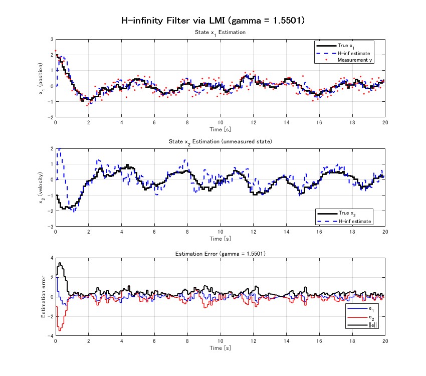
Simulation Result

Continuous-Time H-infinity Filter

For continuous-time systems:

$\displaystyle \dot{x}(t) = Ax(t) + Bu(t) + B_d w(t)$

$\displaystyle y(t) = Cx(t) + Dw(t)$

the continuous-time $H_\infty$ filter takes the form:

$\displaystyle \dot{\hat{x}}(t) = A\hat{x}(t) + Bu(t) + L\bigl(y(t) - C\hat{x}(t)\bigr)$

The design condition for

$\displaystyle \|T_{w \to \tilde{z}}\|_{\infty} < \gamma$

becomes the existence of $P \succ 0$ satisfying:

$\displaystyle (A - LC)^T P + P(A - LC) + P(B_d - LD)\gamma^{-2}(B_d - LD)^T P + C_z^T C_z < 0$

With the substitution $Y = PL$ , this can again be converted to an LMI. This is the continuous-time Bounded Real Lemma applied to the error system.

Comparison: Kalman Filter vs. H-infinity Filter

The Kalman filter and the $H_\infty$ filter represent two fundamentally different approaches to state estimation, each with its own strengths.

Aspect	Kalman Filter	$H_\infty$ Filter
Noise assumption	Gaussian, known covariance (Q, R)	Finite energy, no distribution assumed
Optimality criterion	Minimizes mean-squared error	Minimizes worst-case error-to-disturbance ratio
Design tool	Riccati equation	LMI (convex optimization)
Robustness	Sensitive to incorrect Q, R	Inherently robust
Average performance	Optimal (for Gaussian noise)	Conservative (suboptimal on average)
Worst-case performance	No guarantee	Guaranteed by $\gamma$
Additional design flexibility	Limited	Easy to add constraints (pole placement, structural)

In practice, the Kalman filter tends to give better performance when noise statistics are well known, while the $H_\infty$ filter is preferred when:

The noise characteristics are uncertain
Guaranteed worst-case bounds are required
Additional design constraints must be imposed simultaneously

A useful practical approach is to design both filters and compare their performance: the Kalman filter as a baseline, and the $H_\infty$ filter when robustness is a concern.

Extension to Multi-Rate Systems

In multi-rate sensing environments where sensors have different sampling periods, the $H_\infty$ filter design extends naturally via the periodically time-varying observer framework.

The multi-rate system is modeled using a periodic diagonal selection matrix $S_{k}$ that indicates which sensors are active at each time step. The observer gain $L_{k}$ becomes periodically time-varying with the same frame period $N = \mathrm{lcm}(N_{1}, \ldots, N_{q})$ .

The key advantage of the LMI approach in the multi-rate setting is that:

Periodic Lyapunov matrices $P_{0}, P_{1}, \ldots, P_{N-1}$ can be used in the LMI conditions, providing less conservative results than a single common Lyapunov matrix.
The $\ell_{2}$ -induced norm (the discrete-time counterpart of the $H_\infty$ norm for periodic systems) serves as the appropriate performance measure.
Additional constraints such as pole placement for guaranteed convergence rates can be incorporated as extra LMI conditions.

This framework has been applied to state observer design for multi-rate sensing in IEEE Access (2023), where the observer gains are optimized to minimize the worst-case estimation error over all bounded-energy disturbances.

For the detailed multi-rate observer design with LMI, see: State Observer Under Multi-Rate Sensing Environment and Its Design Using l2-Induced Norm

Design Guidelines

Choosing the Performance Level gamma

The parameter $\gamma$ controls the trade-off between conservatism and feasibility:

A smaller $\gamma$ gives tighter worst-case bounds but may lead to an infeasible LMI (no solution exists).
A larger $\gamma$ is always easier to achieve but provides weaker guarantees.
The optimal $\gamma_{\ast}$ is the smallest value for which the LMI is feasible. This can be found by solving the optimization problem: minimize $\gamma$ subject to the LMI.

Choosing the Estimation Target z

The matrix $C_{z}$ determines which states or linear combinations of states are most important to estimate accurately. Common choices:

$C_{z} = I$ : minimize the overall estimation error for all states equally
$C_{z} = C_{i}$ (a specific row): focus on estimating a particular output or state component
$C_{z}$ as a weighting matrix: prioritize certain states over others based on their importance in the control objective

Combining with Pole Placement

The LMI framework allows adding pole placement constraints alongside the $H_\infty$ condition. For discrete-time systems, requiring all eigenvalues of $A - LC$ to lie within a circle of radius $\bar{r}$ ( $\bar{r} \lt 1$ ) centered at the origin can be expressed as:

$\displaystyle \begin{pmatrix} \bar{r}^2 P & PA - YC \cr (PA - YC)^T & P \end{pmatrix} > 0$

This LMI is added to the $H_\infty$ condition, and both are solved simultaneously. This ensures not only that the worst-case estimation error is bounded, but also that the estimation error converges at a guaranteed rate.

Multi-Rate State Observer — H. Okajima, Y. Hosoe and T. Hagiwara, State Observer Under Multi-Rate Sensing Environment and Its Design Using l2-Induced Norm, IEEE Access (2023). Applies the LMI-based $H_\infty$ -type design framework to multi-rate sensing systems with periodic Lyapunov matrices for optimal observer gain computation.

Multi-Rate Observer-Based Feedback Control — H. Okajima, K. Arinaga and A. Hayashida, Design of observer-based feedback controller for multi-rate systems with various sampling periods using cyclic reformulation, IEEE Access (2023). Extends the $H_\infty$ -type multi-rate observer to a complete feedback control system with guaranteed performance.

Multi-Rate Kalman Filter — H. Okajima, LMI Optimization Based Multirate Steady-State Kalman Filter Design, arXiv:2602.01537 (2026, submitted). Extends the LMI framework to Kalman filter design for multi-rate systems, including mixed H₂/l₂-induced norm design that balances average and worst-case performance.

Model Error Compensator (MEC) — When there is a significant gap between the nominal model and the actual plant, the Model Error Compensator can be combined with the $H_\infty$ filter to further enhance robustness of the observer-based control system.

MATLAB Code

GitHub (H-infinity Filter): MATLAB_state_observer/04_hinf_filter
MATLAB File Exchange (Multi-Rate Observer): State Estimation under Multi-Rate Sensing: IEEE ACCESS 2023
GitHub (LMI basics): MATLAB Fundamental Control LMI
GitHub (Multi-Rate Kalman Filter): multirate-kalman-filter

Self-Introduction

Hiroshi Okajima — Associate Professor, Graduate School of Science and Technology, Kumamoto University. Member of SICE, ISCIE, and IEEE.

www.control-theory.com / Blog / YouTube / GitHub

If you found this article helpful, please consider bookmarking or sharing it.

HinfinityFilter #H-infinity Filter #RobustEstimation #StateObserver #StateEstimation #LMI #LinearMatrixInequality #ControlEngineering #MultiRateSystems #SensorFusion #MATLAB