https://blog.control-theory.com/entry/2024/10/19/170411

Linear matrix inequalities (LMIs) and controller design

The method using Linear Matrix Inequality (LMI) is one of the most powerful controller design methods in the field of control engineering. The usefulness of controller design using LMI is summarized as follows:

Various design specifications and constraints can be expressed using LMI.
Problems formulated with LMI can be solved accurately through efficient convex optimization algorithms.
It is easy to handle problems with multiple constraints and objectives.

Due to these three features, various types of control problems can be formulated as LMI problems, and the controller parameters are derived by solving these LMI problems.

About LMIs

Here, we first explain what LMI is. For a given symmetric matrix $n\times n$ $X$ , $X$ > $0$ means that $X$ is positive definite. In this case, the value of $\xi^T X \xi$ for any (non-zero) real vector $\xi \in R^{n\times 1}$ will always be positive. On the other hand, $X\geq 0$ means semi-positive definite, and $X$ < $0$ means negative definite. A matrix $X$ where the value of $\xi^T X \xi$ can be both positive and negative is called indefinite. Additionally, expressions like $X$ > $0$ , $X$ < $0$ , and $X\geq 0$ are called matrix inequalities. Now, let us consider the following matrix-valued function, which is defined by the symmetric matrices $X_i = X_i^T (i = 0,\cdots,N)$ and the $N$ dimensional vector variable $x = \left(x_1,\cdots,x_N\right)$ :

\begin{equation} X(x)=X_0 + X_1 x_1 + \cdots + X_N x_N \end{equation}

In this case, $X(x)$ is an affine function with respect to the variable $x$ , and conditions like $X(x)$ > $0$ and $X(x)\geq 0$ are LMIs. Here, we deal with the problem of finding $x$ that satisfies these inequality conditions. In particular, since we deal with problems that aim to optimize a certain index (evaluation function value) in controller parameter design, we consider the following problem:

\begin{equation} \min c^T x \, \mathrm{s.t.}\, X(x) \geq 0 \end{equation}

The above formulation is called a semi-definite programming problem, and if the problem setting is solvable, it is possible to obtain a globally optimal solution. This problem seeks to find $x$ that minimizes the value of $c^T x$ while satisfying the constraint $X(x) \geq 0$ . LMI problems have proposed solution algorithms using interior-point methods, which enable efficient solutions (usefulness 2).

If control specifications and constraints can be described using LMI, it becomes easy to simultaneously consider multiple constraints. Specifically, when two specifications $X_1(x)$ > $0$ and $X_2(x)$ > $0$ are given, they can be combined into the following single LMI condition concerning $\bar X(x)$ :

\begin{equation} \bar X(x) := \left[\begin{array}{cc}X_1(x) & 0\\0 & X_2(x)\end{array}\right] > 0 \end{equation}

Additionally, as an equivalent condition, the LMI condition can also be written as follows:

\begin{equation} -\left[\begin{array}{cc}X_1(x) & 0\\0 & X_2(x)\end{array}\right] < 0 \end{equation}

Here, we considered the case where two specifications were given, but more specifications can be combined simultaneously (usefulness 3). In control design, various design specifications are often given, and LMI is highly compatible with controller design.

Solution Example of LMI Problem

Here, we will describe the process of control design using LMI through an example of a controller design.

First, the control target is given by the following continuous-time state equation.
\begin{equation} \dot x = A x + B u + B_2 w \end{equation}

\begin{equation} y = Cx \end{equation}
$x$ represents the state, $u$ is the control input, $w$ is the disturbance, and $y$ is the output. The matrices are given as follows.
\begin{equation} A = \left[\begin{array}{ccc} 0 & 1 & 0 \\ 0 & 0 & 1 \\ 2 & -1.2 & 2.3 \end{array}\right], B = \left[\begin{array}{c} 0 \\ 0 \\ 1 \end{array}\right], \end{equation}

\begin{equation}B_2 = \left[\begin{array}{c} 5 \\ 1 \\ -2 \end{array}\right], C = \left[\begin{array}{ccc} -1 & 5 & 0 \end{array}\right] \end{equation}
Here, we consider the problem of finding a controller $u = -K x$ that minimizes the $L_2$ induced norm (the $L_2$ gain) from the disturbance $w$ to the output $y$ , expressed by the following equation.
\begin{equation} \gamma_* = \sup_{w \in L_2} \frac{\|y\|_2}{\|w\|_2} \end{equation}
$\gamma_*$ represents the influence of the disturbance in the worst-case scenario, and if the value of $\gamma_*$ is small, the influence of the disturbance $w$ on the output $y$ is also small.
When feedback control is applied, the control system, which includes the controller to the control target set above, is described as follows.
\begin{equation} \dot x = (A-BK)x + B_2 w \\ y = (C - D_2 K)x \end{equation}
Here, we formulate this problem as an optimization problem using LMI. To optimize the parameters of the controller $K$ , we solve for $P \gt 0$ , $\gamma$ , and $Z$ that satisfy the following LMI.

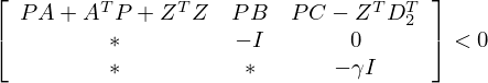
However, $Z^T Z$ is a product of variables, but it can be converted into an LMI using Schur's lemma. The controller $K$ is given by the following equation.

\begin{equation} K = ZP^{-1} \end{equation}

This optimization problem can be solved efficiently using MATLAB. MATLAB provides toolboxes that support the solution of LMI problems, allowing the problem to be described concisely and the solution to be obtained.

Control Specifications Given as LMIs

In this section, various control specifications that can be expressed as LMI conditions are introduced. Although the focus here is on conditions for continuous-time linear time-invariant systems (use case 1.), there are also various LMI conditions available for control specifications concerning discrete-time systems.

Stability and Robust Stability
$L_2$ Induced Norm, $H_\infty$ Norm, and Bounded Realness
Positive Realness
$H_2$ Norm
Peak Value of the Impulse Response
Pole Placement

First, the most fundamental property in constructing a control system is (1:) stability. Stability conditions can be expressed as LMIs. Furthermore, when the control target involves uncertainties, robust stability conditions can also be described as LMIs. Next, the LMI conditions for the (2:) $L_2$ induced norm are given by the inequality conditions described above. The $H_\infty$ norm is equivalent to the $L_2$ induced norm, and for single-input, single-output systems, the $H_\infty$ norm characterizes the peak value in the gain diagram. (3:) Positive realness is a condition related to phase and can also be described as an LMI. Together with the (2:) bounded realness condition, it plays a crucial role in robust control LMI conditions.

Additionally, (4:) the $H_2$ norm and (5:) the peak value of the impulse response, when the system has scalar input, can also be described as LMI conditions. LMI conditions concerning the poles of the control target (6:) analyze whether all poles lie within a designated region. In setting such regions, sector regions, $\alpha$ -stability regions, and circular regions are typically used in combination.

As described above, various types of control specifications can be expressed as LMI conditions, making them useful in control system analysis and design. In particular, conditions (1:) through (3:) have strong affinity with robust control, and LMIs have played a significant role in robust control. When designing a controller that satisfies multiple control specifications, these LMI conditions must be solved simultaneously.

In addition to the control specifications mentioned here, the generalized KYP lemma, which provides frequency-specific characteristics (positive realness, bounded realness) restricted to finite frequencies, can be set as an LMI condition for more detailed design across frequency bands.

Linear matrix inequalities (LMIs) and controller design

About LMIs

Solution Example of LMI Problem

Control Specifications Given as LMIs

Video about LMIs

Playlist

GitHub MATLAB codes

Related article