https://blog.control-theory.com/entry/2024/10/01/143305

This article summarizes state estimators (state observers) for systems represented by state equations. A video explaining the state observer for systems expressed by state equations is provided at the bottom. Observers are also called software sensors because they observe information that cannot be directly measured through computation.

For a comprehensive guide covering Kalman filters, H∞ filters, multi-rate estimation, and other advanced state estimation methods, see the following hub article:

State Observer and State Estimation: A Comprehensive Guide

For an overview of state feedback control, please refer to the following article:

Summary of State Feedback Control and Control Based on State Equations

MATLAB Code: GitHub — MATLAB_state_observer

Overview of State Observers

Let's explain state observers. In control systems, it is not always possible to sense all signals of a system, so it is necessary to estimate the state. In the state equation, variables such as velocity and position are generally considered states, distinct from the observed output. In implementing state feedback using state values, it is necessary to estimate unknown states. For example, if the states are [position] and [velocity], but only [position] is observed, it is necessary to estimate the velocity.

Consider a control object given as shown in the figure, where state feedback control is applied with $u = -Kx$ . State feedback control is one of the most fundamental control methods in the field of control engineering. In state feedback control, it is assumed that all states are used. If estimates are obtained through a state observer, state feedback control can be realized by using these estimates instead.

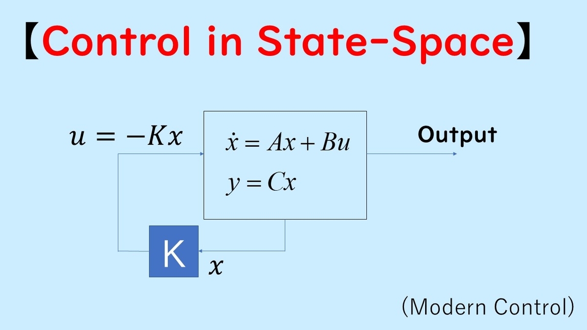
Generally, there is a relationship between the number of states and the observable outputs where the number of states is greater than the number of observable outputs. For using state information in control, a state observer is usually used to estimate the accurate trajectory of the state.

Basic Concept of State Observers

Here we explain the basic concept of observers.

First, when the dynamics of the control object are given as shown in the upper part of the figure, a copy of the control object with the same A, B, C matrices is created on a computer. This is called a mathematical model. When control input is applied to the control object, an output appears, and if the same input is applied to the copy of the control object, the state of the mathematical model behaves similarly to the state of the control object.

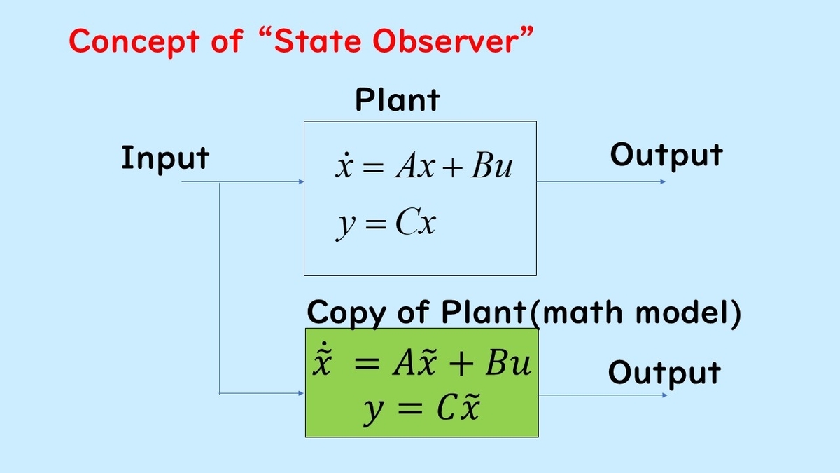
Relationship Between States of Control Object and Model (Stable)

If the poles of the A matrix of the system are stable and the initial values of the state of the control object and the mathematical model are the same, the states of the control object and the mathematical model will completely match at all times in a disturbance-free environment.

Even if the initial values of the states do not match, if A is stable, the influence of these initial values decreases over time, so after some time, the state of the control object and the state of the mathematical model, which is a copy of the control object, become close.

Therefore, the state of the mathematical model can be considered the state of the control object and used in state feedback control.

Furthermore, by using the deviation between the output of the control object and the output of the copy of the control object in feedback, the accuracy of convergence can be improved (see the figure below).

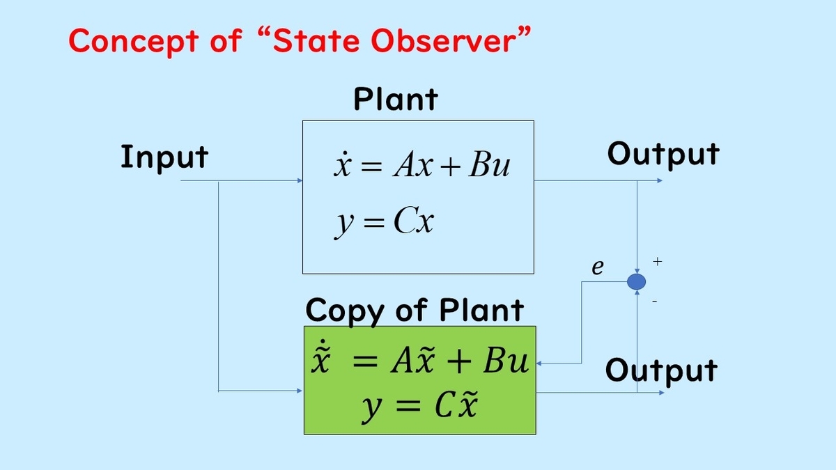
This is the concept of the observer.

Formulation of Observer (Continuous-Time)

Consider a continuous-time LTI plant:

$\displaystyle \dot{x}(t) = Ax(t) + Bu(t)$

$\displaystyle y(t) = Cx(t)$

where $x(t) \in \mathbb{R}^{n}$ is the state, $u(t)$ is the input, and $y(t)$ is the observed output. In many practical cases, the number of outputs is smaller than the number of states ( $\dim(y) < \dim(x)$ ), so not all states can be measured directly.

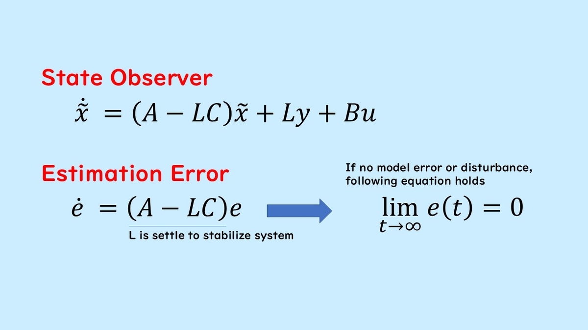
The continuous-time Luenberger observer is given by:

$\displaystyle \dot{\tilde{x}}(t) = A\tilde{x}(t) + Bu(t) + L\bigl(y(t) - C\tilde{x}(t)\bigr)$

Here, $\tilde{x}(t)$ is the estimated state and $L$ is the observer gain matrix.

Defining the estimation error $e(t) = x(t) - \tilde{x}(t)$ , the error dynamics become:

$\displaystyle \dot{e}(t) = (A - LC)\,e(t)$

By choosing $L$ so that all eigenvalues of $A - LC$ have negative real parts (i.e., $A - LC$ is Hurwitz), the estimation error $e(t)$ asymptotically converges to zero. This observer can be designed even if $A$ is unstable, as long as the pair $(C, A)$ is observable.

This is the mechanism of the state observer: since the estimation error converges to zero, the estimated state can be used in place of the true state for control.

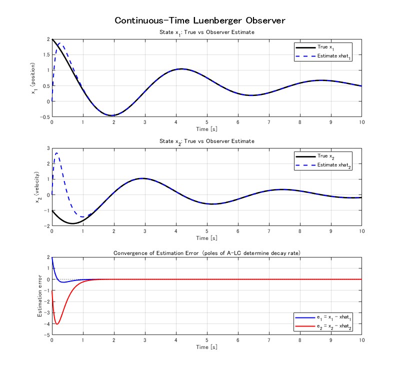
Dynamics of Estimation Error in State Observer

MATLAB code: The continuous-time observer example (main_continuous.m) demonstrates this formulation using a mass-spring-damper system with $n = 2$ states (position and velocity), where only position is measured. The observer gain $L$ is designed via pole placement so that the observer poles are 3–5 times faster than the plant poles.

State Observer for Continuous-time System

Formulation of Observer (Discrete-Time)

For digital implementation, the discrete-time version of the observer is more commonly used. Consider a discrete-time LTI plant:

$\displaystyle x(k+1) = Ax(k) + Bu(k)$

$\displaystyle y(k) = Cx(k)$

The discrete-time Luenberger observer is:

$\displaystyle \hat{x}(k+1) = A\hat{x}(k) + Bu(k) + L\bigl(y(k) - C\hat{x}(k)\bigr)$

The estimation error $e(k) = x(k) - \hat{x}(k)$ satisfies:

$\displaystyle e(k+1) = (A - LC)\,e(k)$

For convergence, all eigenvalues of $A - LC$ must lie inside the unit circle (i.e., $A - LC$ is Schur stable). The closer the observer poles are to the origin, the faster the estimation error converges to zero.

MATLAB code: The discrete-time observer example (main_discrete.m) compares two observer designs — slow poles at $(0.5,\; 0.4)$ and fast poles at $(0.1,\; 0.05)$ — demonstrating how pole placement affects convergence speed. The unmeasured velocity state $x\_{2}$ is accurately estimated from the position measurement alone.

Simulation: Effect of Observer Pole Placement

The MATLAB codes provided in the GitHub repository demonstrate the observer behavior using a mass-spring-damper system ( $m = 1$ , $c = 0.5$ , $k = 2$ ).

Continuous-time example (main_continuous.m):

The plant has states $x = \lbrack q,\; \dot{q} \rbrack^{T}$ (position and velocity), with only position measured ( $C = \lbrack 1,\; 0 \rbrack$ ). The observer poles are placed at $-5$ and $-6$ , which are significantly faster than the plant poles (approximately $-0.25 \pm 1.39j$ ). The estimation error converges rapidly to zero.

Discrete-time example (main_discrete.m):

The same system is discretized with sampling period $T\_{s} = 0.1$ s. Two observer designs are compared:

Slow observer: poles at $0.5$ and $0.4$ — moderate convergence
Fast observer: poles at $0.1$ and $0.05$ — rapid convergence

Both observers successfully estimate the unmeasured velocity state from position measurements, but the fast observer achieves convergence in approximately 0.5 s while the slow observer requires about 2 s.

Observer-Based System

A system using both a state observer and state feedback is called an observer-based system (observer-based state feedback control).

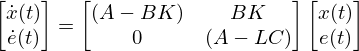
The closed-loop system order is $2n$ . The poles are determined by two independent sets: the observer poles (eigenvalues of $A - LC$ ) and the feedback controller poles (eigenvalues of $A - BK$ ). This feature, where the observer and controller can be independently designed, is called the separation principle.

In an observer-based system, the control input is $u = -K\tilde{x}$ , using the estimate $\tilde{x}$ instead of the true state. Therefore, the observer error should converge quickly, so the observer poles are typically placed further into the stable region than the controller poles.

Continuous-time: observer poles further to the left in the complex plane
Discrete-time: observer poles closer to the origin in the unit disk

Relationship Between Observer and Feedback Control Poles

For the MATLAB code demonstrating observer-based state feedback control, see 02_observer_based_control/ in the GitHub repository.

When Do You Need a State Observer?

State observers are essential in many practical situations:

Unmeasured states: When sensors can only measure some of the system states (e.g., position is measured but velocity is not), an observer estimates the remaining states.
Noisy measurements: By combining the mathematical model with measurements, observers can provide smoother state estimates than raw sensor signals. For stochastic noise, the Kalman filter is the optimal estimator.
Multi-rate sensing: When sensors operate at different sampling rates, specialized observers are required. See Multi-Rate Observer for details.
Cost reduction: Replacing expensive sensors with a software observer (using a cheaper sensor combined with a mathematical model) can reduce system costs while maintaining control performance.

Practical Design Procedure

The steps to design a Luenberger observer are summarized as follows:

Obtain the plant model $(A, B, C)$ : through physical modeling or system identification. For continuous-time models, discretization may be needed.
Check observability: verify that the pair $(C, A)$ is observable (i.e., the observability matrix has full rank).
Choose observer poles: place them faster than the controller poles, but not excessively fast (to avoid noise amplification).
Compute the observer gain $L$ : using pole placement (e.g., MATLAB place command) or LMI-based optimization.
Validate via simulation: confirm that the estimation error converges as expected.

When the plant model is inaccurate, the Model Error Compensator (MEC) can be combined with the observer to improve robustness.

Advanced State Estimation Methods

The Luenberger observer described in this article is the most fundamental state estimator. For more advanced methods, see the hub article:

State Observer and State Estimation: A Comprehensive Guide

Topics covered include:

Kalman Filter — optimal estimation under Gaussian noise
H-infinity Filter — robust estimation using LMI optimization
Multi-Rate Observer — estimation with sensors at different sampling rates
MCV Observer — robust estimation against sensor outliers

MATLAB Code

The MATLAB codes for this article are available in the following GitHub repository:

GitHub: MATLAB_state_observer
- 01_luenberger_observer/ — Luenberger observer (continuous-time and discrete-time)
- 02_observer_based_control/ — Observer-based state feedback control

The following video explains the state observer for a system expressed by state equations.

youtu.be